Tracking Particles and Measuring How They Move

Small particles suspended in water move randomly because water molecules keep bumping into them (Brownian motion). By following each particle through a video, we can measure this motion and ask whether it is purely random.

This notebook tracks colloidal particles in water (the bulk_water dataset) with the Trackpy library [21], using a single call, spice.segmentation.run_trackpy().

JuSPICE Modules and Classes

• juspice.io: load_frame_sequence, save_data, SPICEData

• juspice.segmentation_module: UNetSegmentationAccessor (via spice.segmentation)

• juspice.synth_data_module: ConfigLoader

• juspice.tracking: Tracker

from juspice.tracking import Tracker

tracker = Tracker(include_metadata=True, notes='Particle tracking with trackpy')

tracker.recording_start()

/Users/amir/GIT_repositories/juspice_pre_release/venvs/.venv/lib/python3.12/site-packages/tqdm/auto.py:21: TqdmWarning: IProgress not found. Please update jupyter and ipywidgets. See https://ipywidgets.readthedocs.io/en/stable/user_install.html
  from .autonotebook import tqdm as notebook_tqdm

# --------- Block 0: Setup ----------

# Standard library
from pathlib import Path
import sys
import os
import json
import logging
import shutil

# Third-party
import numpy as np
import matplotlib.pyplot as plt

# JuSPICE
from juspice.io import load_frame_sequence, save_data, SPICEData
from juspice.synth_data_module import ConfigLoader

# Paths
try:
    notebook_dir = Path(__file__).resolve().parent
except Exception:
    notebook_dir = Path.cwd()

cur = notebook_dir
repo_root = None
for _ in range(6):
    if (cur / 'juspice').exists() or (cur / 'pyproject.toml').exists():
        repo_root = cur
        break
    if cur.parent == cur:
        break
    cur = cur.parent
if repo_root is None:
    repo_root = notebook_dir
if str(repo_root) not in sys.path:
    sys.path.insert(0, str(repo_root))

tracker.recording_stop()

From images to trajectories

Tracking has two parts. First, particles are detected in each frame as roughly round spots of a given size (diameter) and minimum brightness (minmass). Then detections in consecutive frames are linked into trajectories, assuming the particle has moved only a short distance (link_search_range). Trackpy uses the method of Crocker and Grier (1996) [46] for this.

run_trackpy() also removes very short trajectories (stub_threshold), filters out particles that are too faint, too large, or not round enough, and subtracts any overall drift of the sample.

Mean squared displacement (MSD)

To describe the motion, we compute how far particles move, on average, during a time interval τ. Squaring the displacement makes all directions count positively:

\[\text{MSD}(\tau) = \langle |\mathbf{r}(t+\tau) - \mathbf{r}(t)|^2 \rangle\]

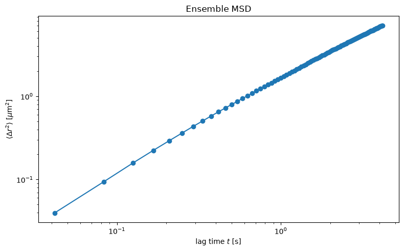
For random (Brownian) motion in two dimensions, MSD = 4Dτ [47], where D is the diffusion coefficient. On a log–log plot, the slope of the MSD tells us the type of motion:

• slope ≈ 1: random diffusion

• slope > 1: directed motion, e.g. flow

• slope < 1: hindered or confined motion

microns_per_pixel and fps convert pixels and frames into micrometres and seconds.

tracker.recording_start()

# --------- Block 1: Load frame sequence and run Trackpy ----------

config_path = os.path.join(repo_root, 'notebooks', 'notebooks_parameters.yaml')
config = ConfigLoader(config_path)

bulk_water_params = config.get_dataset_params('bulk_water')
data_dir = os.path.join(repo_root, bulk_water_params['training_images_dir'])

# TrackPy operates on frame sequences.  load_frame_sequence() loads all frames
# as a stacked (n_frames, H, W) array — the natural SPICEData-native entry point.
# The frames are ordered by the first numeric run embedded in each filename.
# `spice` is just a variable name for the SPICEData instance load_data()
# returns here — any name would work; we use `spice` throughout these
# notebooks as an intuitive nod to JuSPICE / SPICEData.
spice = load_frame_sequence(data_dir)
print(f'Loaded {spice.n_frames} frames from {data_dir}')
print(f'dataset_type: {spice.dataset_type!r}, data.shape: {spice.data.shape}')

# run_trackpy() runs the full pipeline:
#   batch detection → trajectory linking → stub filtering →
#   optional quality filtering → drift correction → ensemble MSD.
# spice.data (n_frames, H, W) is used directly; channel=1 picks the green
# channel if frames are multi-channel RGB.
msd_spice = spice.segmentation.run_trackpy(
    diameter=11,
    minmass=20,
    max_frames=300,
    link_search_range=5,
    memory=3,
    stub_threshold=25,
    mass_min=50,
    size_max=2.6,
    ecc_max=0.3,
    microns_per_pixel=100 / 285.,
    fps=24,
    invert=True,
    channel=1,  # green channel if RGB
)

print(f'Ensemble MSD computed: {len(msd_spice.data)} lag-time points')
print(f'Particles tracked: {msd_spice.metadata["num_particles_filtered"]}')

Frame 299: 624 trajectories present.
Ensemble MSD computed: 100 lag-time points
Particles tracked: 1059

tracker.recording_stop()

tracker.recording_start()

Reading the MSD plot

Each point is the MSD averaged over all tracked particles for one time lag. A straight line with slope close to 1 is consistent with Brownian motion. From that line, D can be estimated.

Be careful at the ends of the curve:

• At the shortest lags, uncertainty in locating each particle adds a constant offset, which flattens the curve and can look like hindered motion.

• At the longest lags, fewer trajectory segments are available, so the values scatter more. Residual drift can also bend the curve upward.

# --------- Block 2: Visualize ensemble MSD ----------

lag_times = msd_spice.metadata['lag_times']
msd_values = msd_spice.data

fig, ax = plt.subplots(figsize=(8, 5))
ax.plot(lag_times, msd_values, 'o-')
ax.set_xscale('log')
ax.set_yscale('log')
ax.set(
    ylabel=r'$\langle \Delta r^2 \rangle$ [$\mu$m$^2$]',
    xlabel='lag time $t$ [s]',
    title='Ensemble MSD',
)
plt.tight_layout()
plt.show()

print(f'n_frames processed: {msd_spice.metadata["n_frames_processed"]}')
print(f'particles (before filter): {msd_spice.metadata["num_particles"]}')
print(f'particles (after filter):  {msd_spice.metadata["num_particles_filtered"]}')

n_frames processed: 300
particles (before filter): 1505
particles (after filter):  1059

Check the intermediate steps

The final curve depends on every earlier step, so it is worth checking them:

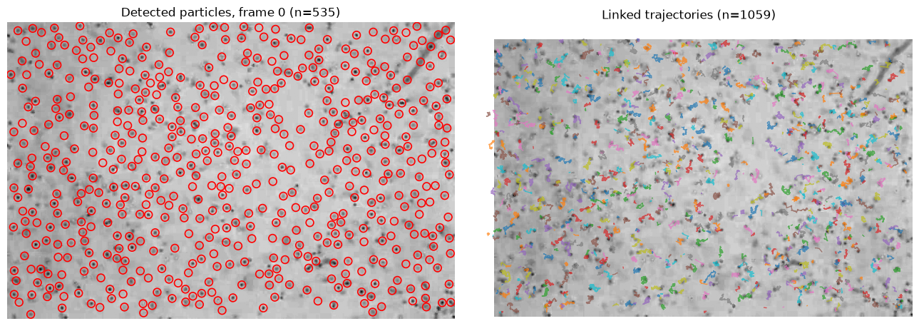
• Left: the particles detected in the first frame. Missed or false detections would suggest adjusting diameter or minmass.

• Right: the linked trajectories.

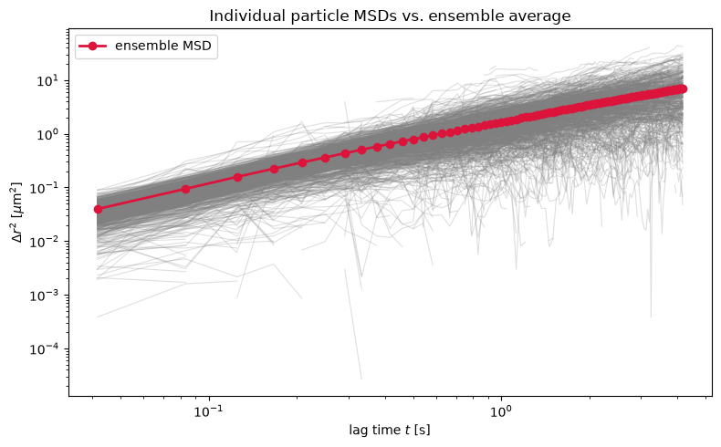
• Second figure: the MSD of each individual particle (grey) compared with the average (red). The spread shows how much single particles differ from the average.

# --------- Block 2b: Visualize intermediate tracking results ----------

# msd_spice.extra carries three intermediate results from
# run_trackpy()'s pipeline, not just the final ensemble MSD — no
# re-tracking needed to visualize them.
import trackpy as tp

features = msd_spice.extra['detected_features']
trajectories = msd_spice.extra['trajectories']
first_frame = msd_spice.extra['first_frame']
microns_per_pixel = msd_spice.metadata['microns_per_pixel']
fps = msd_spice.metadata['fps']

fig, axes = plt.subplots(1, 2, figsize=(13, 6))

# Left: particles Trackpy actually detected in the first processed frame
frame0_features = features[features['frame'] == 0]
axes[0].imshow(first_frame, cmap='gray')
axes[0].scatter(
    frame0_features['x'], frame0_features['y'],
    s=60, facecolors='none', edgecolors='red', linewidths=1.2,
)
axes[0].set_title(f'Detected particles, frame 0 (n={len(frame0_features)})')
axes[0].axis('off')

# Right: the linked, filtered, drift-corrected trajectories
axes[1].imshow(first_frame, cmap='gray')
for _, group in trajectories.groupby(trajectories['particle']):
    axes[1].plot(group['x'], group['y'], linewidth=1, alpha=0.7)
n_particles = trajectories['particle'].nunique()
axes[1].set_title(f'Linked trajectories (n={n_particles})')
axes[1].axis('off')

plt.tight_layout()
plt.show()

# Individual (per-particle) MSD, before ensemble averaging — shows how
# much particle-to-particle variation the ensemble MSD plot smooths over.
individual_msd = tp.imsd(trajectories, microns_per_pixel, fps)

fig, ax = plt.subplots(figsize=(8, 5))
ax.plot(
    individual_msd.index, individual_msd,
    color='gray', alpha=0.25, linewidth=0.8,
)
ax.plot(lag_times, msd_values, 'o-', color='crimson', linewidth=2, label='ensemble MSD')
ax.set_xscale('log')
ax.set_yscale('log')
ax.set(
    xlabel='lag time $t$ [s]',
    ylabel=r'$\Delta r^2$ [$\mu$m$^2$]',
    title='Individual particle MSDs vs. ensemble average',
)
ax.legend()
plt.tight_layout()
plt.show()

tracker.recording_stop()

tracker.recording_start()

Save and review

We save the ensemble MSD and print the recorded pipeline.

# --------- Block 3: Save ----------

# msd_spice IS already the SPICEData returned by spice.segmentation.run_trackpy()
# — no manual wrapping needed. It carries the ensemble MSD and shares spice's
# history lineage.
# This folder holds several notebooks, so save_data()'s automatic
# notebook-name detection would be ambiguous when run outside a live
# Jupyter session (e.g. via nbconvert) — pass output_stem explicitly
# to always land on this notebook's own files. See
# docs/repository_structure.rst.
stem = 'example_trackpy'
save_data(
    msd_spice,
    output_stem=str(notebook_dir / stem),
)
print(f'Data:           {os.path.join(notebook_dir, stem + ".npy")}')
print(f'JSON sidecar:   {os.path.join(notebook_dir, stem + ".json")}')
print(f'History script: {os.path.join(notebook_dir, stem + "_history.py")}')

Data:           /Users/amir/GIT_repositories/juspice_pre_release/notebooks/segmentation/example_trackpy.npy
JSON sidecar:   /Users/amir/GIT_repositories/juspice_pre_release/notebooks/segmentation/example_trackpy.json
History script: /Users/amir/GIT_repositories/juspice_pre_release/notebooks/segmentation/example_trackpy_history.py

tracker.recording_stop()

tracker.recording_start()

# --------- Block 4: Inspect human-readable history ----------

# msd_spice.history.to_lines() reconstructs the full tracking pipeline
# applied to this SPICEData object into readable, runnable code: the
# initial load_frame_sequence(...) call followed by
# spice.segmentation.run_trackpy(...) with all runtime argument values
# (diameter, minmass, link_search_range, stub_threshold, etc.), and
# a trailing save_data(msd_spice).
readable_lines = msd_spice.history.to_lines()

print('Reconstructed tracking pipeline for this SPICEData object:')
print('\n'.join(readable_lines))

Reconstructed tracking pipeline for this SPICEData object:
import juspice
spice = juspice.io.load_frame_sequence('/Users/amir/GIT_repositories/juspice_pre_release/Sample_data/Train_test_images/bulk_water')
msd_spice = spice.segmentation.run_trackpy(diameter=11, minmass=20, n_frames_processed=300, link_search_range=5, stub_threshold=25)
juspice.io.save_data(spice)

tracker.recording_stop()