From an Image Folder to a Time Series

A microscopy video is often saved as a folder of separate image files. This notebook loads such a folder as one ordered dataset and reduces each frame to a single number, turning the video into a curve that is easy to inspect.

The data are 73 frames from an in-situ transmission electron microscopy (TEM) [4] video of a SiO₂ electrode taking up lithium (lithiation).

JuSPICE Modules and Classes

• juspice.io: load_frame_sequence, save_data, SPICEData

• juspice.clustering_module: ClusteringAccessor (via spice.clustering)

• juspice.tracking: Tracker

from juspice.tracking import Tracker

tracker = Tracker(
    include_metadata=True, notes='Dataset creation from SiO2 lithiation frames'
)

tracker.recording_start()

/Users/amir/GIT_repositories/juspice_pre_release/venvs/.venv/lib/python3.12/site-packages/tqdm/auto.py:21: TqdmWarning: IProgress not found. Please update jupyter and ipywidgets. See https://ipywidgets.readthedocs.io/en/stable/user_install.html
  from .autonotebook import tqdm as notebook_tqdm

# --------- Block 0: Setup ----------

# Standard library
from pathlib import Path
import sys
import os

# Third-party
import numpy as np
import matplotlib.pyplot as plt

# JuSPICE
from juspice.io import load_frame_sequence, save_data, SPICEData

# Paths
try:
    notebook_dir = Path(__file__).resolve().parent
except Exception:
    notebook_dir = Path.cwd()

cur = notebook_dir
repo_root = None
for _ in range(6):
    if (cur / 'juspice').exists() or (cur / 'pyproject.toml').exists():
        repo_root = cur
        break
    if cur.parent == cur:
        break
    cur = cur.parent
if repo_root is None:
    repo_root = notebook_dir
if str(repo_root) not in sys.path:
    sys.path.insert(0, str(repo_root))

tracker.recording_stop()

Load the frames

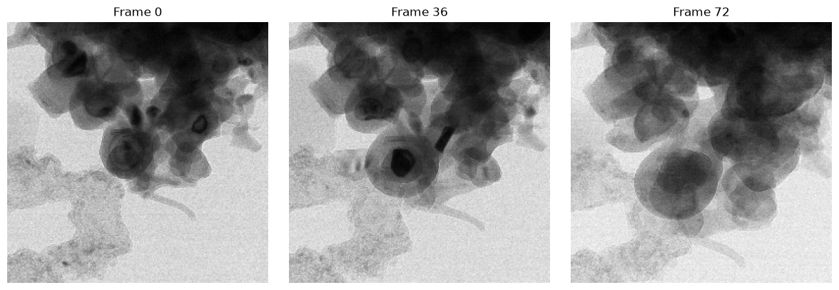
load_frame_sequence() stacks all images in the folder into one array of shape (frames, height, width). The frames are ordered by the first number in each file name.

tracker.recording_start()

# --------- Block 1: Load frame sequence ----------

frames_dir = os.path.join(
    repo_root, 'Sample_data', 'Train_test_images', 'SiO2_lithiation', 'images', 'train'
)
# `spice` is just a variable name for the SPICEData instance load_data()
# returns here — any name would work; we use `spice` throughout these
# notebooks as an intuitive nod to JuSPICE / SPICEData.
spice = load_frame_sequence(frames_dir)

print(f'Loaded {spice.n_frames} frames from {frames_dir}')
print(
    f'dataset_type: {spice.dataset_type!r}, data.shape: {spice.data.shape}, '
    f'dtype: {spice.data.dtype}'
)

fig, axes = plt.subplots(1, 3, figsize=(12, 4))
for ax, idx in zip(axes, (0, spice.n_frames // 2, spice.n_frames - 1)):
    ax.imshow(spice.frames[idx], cmap='gray')
    ax.set_title(f'Frame {idx}')
    ax.axis('off')
plt.tight_layout()
plt.show()

Loaded 73 frames from /Users/amir/GIT_repositories/juspice_pre_release/Sample_data/Train_test_images/SiO2_lithiation/images/train
dataset_type: 'multiple_frames', data.shape: (73, 256, 256), dtype: uint8

tracker.recording_stop()

Count regions in every frame

Watershed segmentation [28] splits an image into regions around bright or dark centres, much like water filling separate basins. It works on one image at a time, so we loop over the frames and store the number of regions found in each.

tracker.recording_start()

# --------- Block 2: Watershed clustering per frame ----------

FOOTPRINT_SIZE = 15
MIN_DISTANCE = 10

n_clusters = []
for frame in spice.frames:
    frame_spice = SPICEData(
        data=frame, metadata={}, data_type='array', source_path=spice.source_path
    )
    ws_spice = frame_spice.clustering.watershed_clustering(
        footprint_size=FOOTPRINT_SIZE, min_distance=MIN_DISTANCE
    )
    n_clusters.append(int(ws_spice.data.max()))

feature_spice = SPICEData(
    data=np.array(n_clusters, dtype=np.int32),
    metadata={**spice.metadata, 'feature': 'watershed_cluster_count',
              'footprint_size': FOOTPRINT_SIZE, 'min_distance': MIN_DISTANCE},
    data_type='array',
    source_path=spice.source_path,
    extra=dict(spice.extra),
    history=spice.history,
)
print(f'Cluster-count time series: shape={feature_spice.data.shape}, '
      f'min={feature_spice.data.min()}, max={feature_spice.data.max()}')

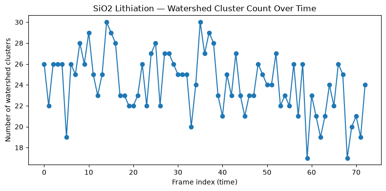
Cluster-count time series: shape=(73,), min=17, max=30

tracker.recording_stop()

Plot the count over time

Since the frames are in recording order, the frame index acts as a time axis. The curve shows how the number of watershed regions changes during the video.

Keep in mind that this count depends on the segmentation settings (FOOTPRINT_SIZE, MIN_DISTANCE). It is an image measure, not a direct count of physical particles.

tracker.recording_start()

# --------- Block 3: Plot cluster-count time series ----------

time_axis = np.arange(len(feature_spice.data))

fig, ax = plt.subplots(figsize=(8, 4))
ax.plot(time_axis, feature_spice.data, 'o-')
ax.set(
    xlabel='Frame index (time)',
    ylabel='Number of watershed clusters',
    title='SiO2 Lithiation — Watershed Cluster Count Over Time',
)
plt.tight_layout()
plt.show()

tracker.recording_stop()

Save

save_data() writes the time series (.npy), its metadata (.json), and a replay script (_history.py).

tracker.recording_start()

# --------- Block 4: Save ----------

# Writes <stem>.npy, <stem>.json, and <stem>_history.py next to the notebook
# This folder holds several notebooks, so save_data()'s automatic
# notebook-name detection would be ambiguous when run outside a live
# Jupyter session (e.g. via nbconvert) — pass output_stem explicitly
# to always land on this notebook's own files. See
# docs/repository_structure.rst.
stem = 'io_create_dataset'
save_data(
    feature_spice,
    output_stem=str(notebook_dir / stem),
)
print(f'Data:           {os.path.join(notebook_dir, stem + ".npy")}')
print(f'JSON sidecar:   {os.path.join(notebook_dir, stem + ".json")}')
print(f'History script: {os.path.join(notebook_dir, stem + "_history.py")}')

Data:           /Users/amir/GIT_repositories/juspice_pre_release/notebooks/io/io_create_dataset.npy
JSON sidecar:   /Users/amir/GIT_repositories/juspice_pre_release/notebooks/io/io_create_dataset.json
History script: /Users/amir/GIT_repositories/juspice_pre_release/notebooks/io/io_create_dataset_history.py

tracker.recording_stop()

Review the recorded steps

to_lines() rebuilds the recorded operations as code. The watershed loop is plain Python rather than a recorded JuSPICE call, so it does not appear here; only loading and saving do.

tracker.recording_start()

# --------- Block 5: Inspect human-readable history ----------

readable_lines = feature_spice.history.to_lines()

print('Reconstructed pipeline for this SPICEData object:')
print('\n'.join(readable_lines))

Reconstructed pipeline for this SPICEData object:
import juspice
spice = juspice.io.load_frame_sequence('/Users/amir/GIT_repositories/juspice_pre_release/Sample_data/Train_test_images/SiO2_lithiation/images/train')
juspice.io.save_data(spice)

tracker.recording_stop()