Splitting an Image into Regions with Clustering

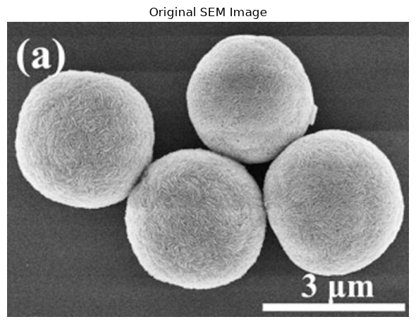
Clustering groups pixels that belong together, without any labelled training examples (unsupervised). Here we apply five clustering methods to the same SEM image and compare the regions they find.

Each method returns a new SPICEData holding a label map, one region number per pixel. The original image stays unchanged.

JuSPICE Modules and Classes

• juspice.io: load_data, save_data, SPICEData

• juspice.clustering_module: ClusteringAccessor (via spice.clustering)

• juspice.tracking: Tracker

from juspice.tracking import Tracker

tracker = Tracker(include_metadata=True, notes='Clustering basics notebook')

tracker.recording_start()

/Users/amir/GIT_repositories/juspice_pre_release/venvs/.venv/lib/python3.12/site-packages/tqdm/auto.py:21: TqdmWarning: IProgress not found. Please update jupyter and ipywidgets. See https://ipywidgets.readthedocs.io/en/stable/user_install.html
  from .autonotebook import tqdm as notebook_tqdm

# --------- Block 0: Setup ----------

# Standard library
from pathlib import Path
import sys
import os
import json
import shutil

# Third-party
import numpy as np
import matplotlib.pyplot as plt
from skimage.segmentation import mark_boundaries
from skimage.color import label2rgb

# JuSPICE
from juspice.io import load_data, save_data, SPICEData

# Paths
try:
    notebook_dir = Path(__file__).resolve().parent
except Exception:
    notebook_dir = Path.cwd()

cur = notebook_dir
repo_root = None
for _ in range(6):
    if (cur / 'juspice').exists() or (cur / 'pyproject.toml').exists():
        repo_root = cur
        break
    if cur.parent == cur:
        break
    cur = cur.parent
if repo_root is None:
    repo_root = notebook_dir
if str(repo_root) not in sys.path:
    sys.path.insert(0, str(repo_root))

tracker.recording_stop()

Load the image

All methods work on a grayscale copy scaled to 0–1 (spice.clustering.image).

tracker.recording_start()

# --------- Block 1: Load ----------

image_path = os.path.join(repo_root, 'Sample_data', 'em', '1b935635dd.png')
# `spice` is just a variable name for the SPICEData instance load_data()
# returns here — any name would work; we use `spice` throughout these
# notebooks as an intuitive nod to JuSPICE / SPICEData.
spice = load_data(image_path)

# spice.clustering.image is the grayscale float [0,1] view used internally;
# it is cached so repeated accesses share the same array.
cluster_image = spice.clustering.image
print(f'Image path: {image_path}')
print(f'Image shape: {cluster_image.shape}')
print(f'Intensity range: [{cluster_image.min():.3f}, {cluster_image.max():.3f}]')

fig, ax = plt.subplots(1, 1, figsize=(6, 5))
ax.imshow(cluster_image, cmap='gray')
ax.set_title('Original SEM Image')
ax.axis('off')
plt.tight_layout()
plt.show()

Image path: /Users/amir/GIT_repositories/juspice_pre_release/Sample_data/em/1b935635dd.png
Image shape: (512, 697)
Intensity range: [0.000, 1.000]

tracker.recording_stop()

Watershed: separating touching particles

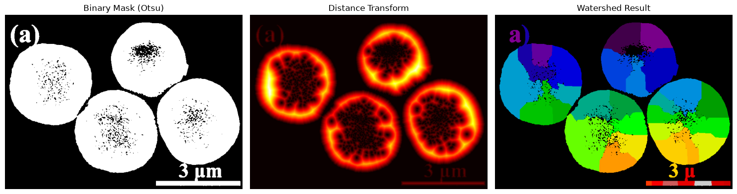
Watershed segmentation [28] is used here in its marker-based form. A threshold first splits bright from dark pixels (left). The distance of each foreground pixel to the background peaks at particle centres (middle). Regions then grow outward from these peaks until they meet (right), which can separate touching particles.

tracker.recording_start()

# --------- Block 2: Watershed ----------

# spice.clustering.watershed_clustering() derives a NEW SPICEData with the
# label array — spice.data is never mutated. Intermediate states
# (binary mask, distance transform, markers) are stored in ws_spice.extra.
ws_spice = spice.clustering.watershed_clustering(footprint_size=60, min_distance=20)
print(f'Number of watershed regions: {int(ws_spice.data.max())}')

fig, axes = plt.subplots(1, 3, figsize=(15, 5))
axes[0].imshow(ws_spice.extra['watershed_binary'], cmap='gray')
axes[0].set_title('Binary Mask (Otsu)')
axes[0].axis('off')
axes[1].imshow(ws_spice.extra['watershed_distance'], cmap='hot')
axes[1].set_title('Distance Transform')
axes[1].axis('off')
axes[2].imshow(ws_spice.data, cmap='nipy_spectral')
axes[2].set_title('Watershed Result')
axes[2].axis('off')
plt.tight_layout()
plt.show()

Number of watershed regions: 35

tracker.recording_stop()

SLIC: superpixels

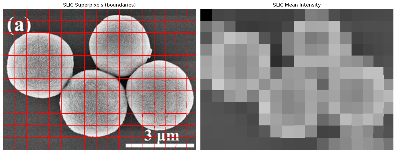
SLIC [30] divides the image into many small patches of similar brightness. Filling each patch with its mean brightness (right) shows how well the patches follow the image.

tracker.recording_start()

# --------- Block 3: SLIC ----------

n_segments = 200
compactness = 10
sigma = 10
slic_spice = spice.clustering.slic_clustering(
    n_segments=n_segments, compactness=compactness, sigma=sigma
)
print(f'Number of superpixels: {int(slic_spice.data.max() + 1)}')

cluster_image = spice.clustering.image  # grayscale float [0,1] — cached
boundaries_vis = mark_boundaries(cluster_image, slic_spice.data, color=(1, 0, 0))
regions_avg = label2rgb(slic_spice.data, image=cluster_image, kind='avg')

fig, (ax0, ax1) = plt.subplots(1, 2, figsize=(14, 6))
ax0.imshow(boundaries_vis)
ax0.set_title('SLIC Superpixels (boundaries)')
ax0.axis('off')
ax1.imshow(regions_avg, cmap='gray')
ax1.set_title('SLIC Mean Intensity')
ax1.axis('off')
plt.tight_layout()
plt.show()

Number of superpixels: 204

tracker.recording_stop()

Felzenszwalb: merging similar neighbours

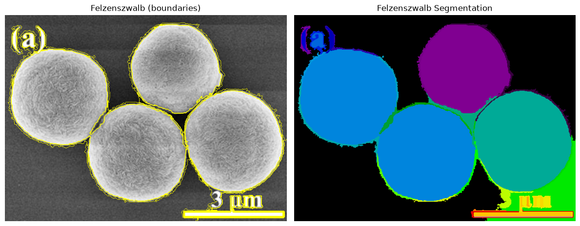
In Felzenszwalb and Huttenlocher’s method [31], neighbouring pixels are merged while their difference is small compared with the variation inside the region. Larger scale values give fewer, larger regions.

tracker.recording_start()

# --------- Block 4: Felzenszwalb ----------

fz_spice = spice.clustering.felzenszwalb_clustering(
    scale=500, sigma=0.5, min_size=100
)
print(f'Number of Felzenszwalb regions: {int(fz_spice.data.max() + 1)}')

cluster_image = spice.clustering.image
fig, axes = plt.subplots(1, 2, figsize=(12, 5))
axes[0].imshow(mark_boundaries(cluster_image, fz_spice.data))
axes[0].set_title('Felzenszwalb (boundaries)')
axes[0].axis('off')
axes[1].imshow(fz_spice.data, cmap='nipy_spectral')
axes[1].set_title('Felzenszwalb Segmentation')
axes[1].axis('off')
plt.tight_layout()
plt.show()

Number of Felzenszwalb regions: 38

tracker.recording_stop()

Otsu: a brightness threshold

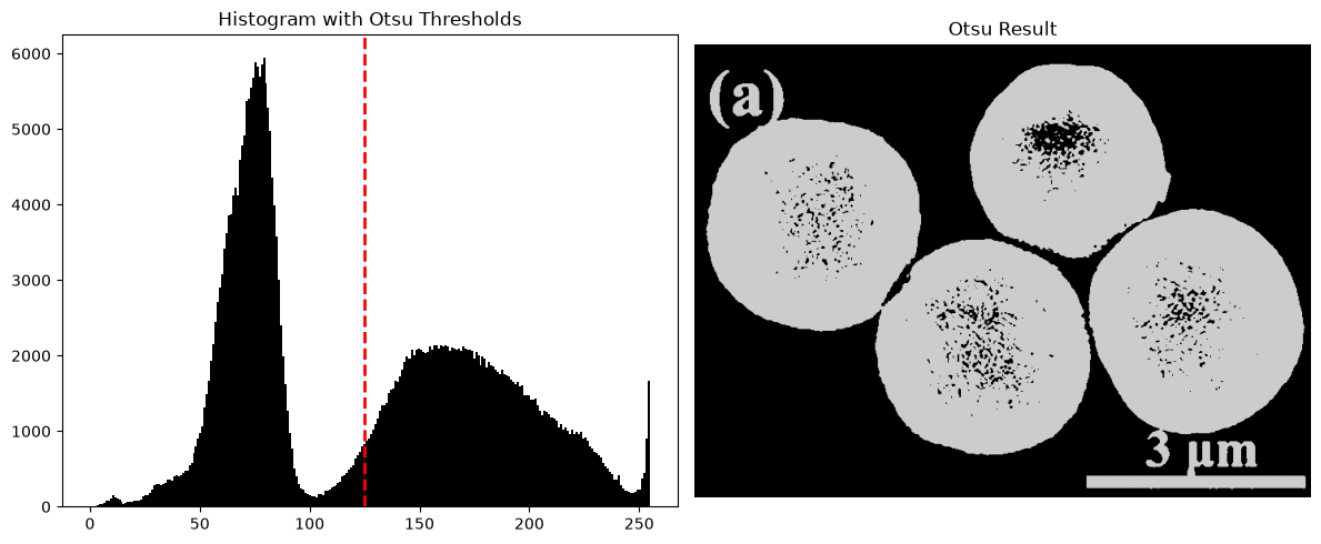
Otsu’s method [9] picks the threshold (red line) that best splits the histogram into dark and bright pixels. It ignores where pixels are located.

tracker.recording_start()

# --------- Block 5: Otsu ----------

otsu_spice = spice.clustering.otsu_multithreshold(n_classes=2)
thresholds = otsu_spice.extra['otsu_thresholds']
print(f'Number of classes: {int(otsu_spice.data.max() + 1)}')
print(f'Otsu thresholds: {thresholds}')

cluster_image = spice.clustering.image
img_uint8 = (cluster_image * 255).astype(np.uint8)
fig, (ax1, ax2) = plt.subplots(1, 2, figsize=(12, 5))
ax1.hist(img_uint8.ravel(), bins=256, color='black')
for t in thresholds:
    ax1.axvline(t * 255, color='red', linewidth=2, linestyle='--')
ax1.set_title('Histogram with Otsu Thresholds')
ax2.imshow(otsu_spice.data, cmap='nipy_spectral')
ax2.set_title('Otsu Result')
ax2.axis('off')
plt.tight_layout()
plt.show()

Number of classes: 2
Otsu thresholds: [0.49023438]

tracker.recording_stop()

Quickshift: brightness and position

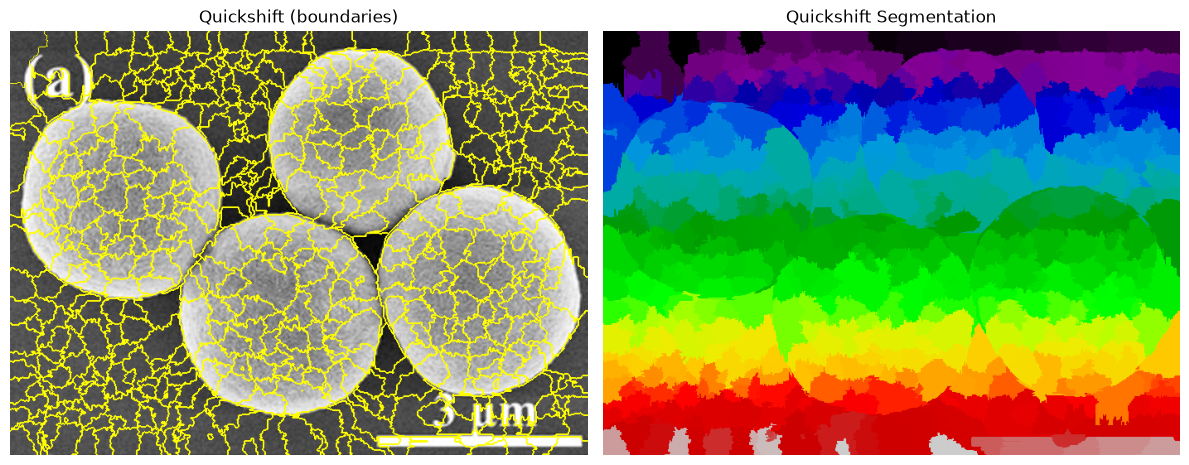
Quickshift [32] groups pixels using both brightness and position. With these settings it produces many small regions, which could be merged later.

Takeaway: Otsu separates by brightness alone, watershed splits touching objects, and SLIC, Felzenszwalb, and Quickshift divide the image into smaller regions of different size and shape.

tracker.recording_start()

# --------- Block 6: Quickshift ----------

qs_spice = spice.clustering.quickshift_clustering(
    kernel_size=5, max_dist=10, ratio=0.5
)
print(f'Number of Quickshift regions: {int(qs_spice.data.max() + 1)}')

cluster_image = spice.clustering.image
fig, axes = plt.subplots(1, 2, figsize=(12, 5))
axes[0].imshow(mark_boundaries(cluster_image, qs_spice.data))
axes[0].set_title('Quickshift (boundaries)')
axes[0].axis('off')
axes[1].imshow(qs_spice.data, cmap='nipy_spectral')
axes[1].set_title('Quickshift Segmentation')
axes[1].axis('off')
plt.tight_layout()
plt.show()

Number of Quickshift regions: 523

tracker.recording_stop()

Save and review

We save the watershed result, print the recorded steps, and check the saved JSON file.

tracker.recording_start()

# --------- Block 7: Save ----------

# ws_spice IS already the SPICEData returned by
# spice.clustering.watershed_clustering() — no manual wrapping needed.
# Add any extra metadata before saving.
ws_spice.metadata.update({
    'method': 'watershed',
    'source_image': image_path,
})

# Writes <stem>.npy, <stem>.json, and <stem>_history.py next to the notebook.
save_data(ws_spice)

stem = 'clustering_basics'
print(f'Data:           {os.path.join(notebook_dir, stem + ".npy")}')
print(f'JSON sidecar:   {os.path.join(notebook_dir, stem + ".json")}')
print(f'History script: {os.path.join(notebook_dir, stem + "_history.py")}')

Data:           /Users/amir/GIT_repositories/juspice_pre_release/notebooks/clustering/clustering_basics.npy
JSON sidecar:   /Users/amir/GIT_repositories/juspice_pre_release/notebooks/clustering/clustering_basics.json
History script: /Users/amir/GIT_repositories/juspice_pre_release/notebooks/clustering/clustering_basics_history.py

# Validate + Inspect
readable_lines = ws_spice.history.to_lines()
print('Reconstructed pipeline:')
print('\n'.join(readable_lines))

# Check the saved JSON: history is a list, one entry per pipeline step.
metadata_path = os.path.join(notebook_dir, 'clustering_basics.json')
if os.path.exists(metadata_path):
    with open(metadata_path, encoding='utf-8') as _fh:
        metadata = json.loads(_fh.read())
    history_lines = metadata.get('history', [])
    assert isinstance(history_lines, list), 'history must be a list'
    assert history_lines, 'history list is empty'
    assert any('load_data(' in line for line in history_lines)
    assert any('clustering.watershed_clustering(' in line for line in history_lines)
    assert any('save_data(' in line for line in history_lines)
    assert 'operations' not in metadata
    assert 'data_shape' in metadata
    assert 'data_dtype' in metadata
    print(f'\nValidation passed. JSON keys: {list(metadata.keys())}')

Reconstructed pipeline:
import juspice
spice = juspice.io.load_data('/Users/amir/GIT_repositories/juspice_pre_release/Sample_data/em/1b935635dd.png')
ws_spice = spice.clustering.watershed_clustering(footprint_size=60, min_distance=20)
slic_spice = spice.clustering.slic_clustering(n_segments=200, compactness=10, sigma=10)
fz_spice = spice.clustering.felzenszwalb_clustering(scale=500, sigma=0.5, min_size=100)
otsu_spice = spice.clustering.otsu_multithreshold(n_classes=2)
qs_spice = spice.clustering.quickshift_clustering(kernel_size=5, max_dist=10, ratio=0.5)
juspice.io.save_data(spice)

Validation passed. JSON keys: ['source_path', 'data_type', 'import_timestamp', 'version_info', 'dataset_metadata', 'history', 'dataset_type', 'data_shape', 'data_dtype', 'n_frames']

tracker.recording_stop()