I/O and History Tracking

← Back to Notebook Examples

notebooks/io/io_create_dataset.ipynb

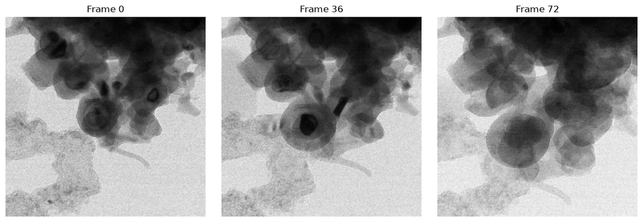
Builds a JuSPICE dataset from a folder of real image frames, then turns it into a single number-per-frame time series — with a Tracker and recording_start()/recording_stop() blocks capturing the code used throughout. The 73 in-situ TEM frames in Sample_data/Train_test_images/SiO2_lithiation/images/train load as one ordered dataset_type='multiple_frames' SPICEData via load_frame_sequence(). A loop then runs marker-based watershed segmentation (spice.clustering.watershed_clustering()) on every frame, counts how many clusters each frame has, and stores that count-per-frame series in a new SPICEData — which gets plotted and saved, along with a session-level history script and per-dataset reproducibility files (.npy, .json, _history.py). Covers JuSPICE’s two-track history system: literal code capture via Tracker, and structured operation recording via DatasetHistory.

notebooks/io/io_afm1.ipynb

Loads a Bruker AFM .spm scan with load_data(), which stacks every channel on the shared pixel grid into one (height, width, n_channels) SPICEData.data array, with channel names in spice.metadata['channel_names']. Shows all channels, levels the Height Sensor channel with pySPM’s own .correct_plane() (the raw pySPM.SPM_image objects stay available in spice.extra['channels']), then pulls out one channel and runs it through the standard spice.preprocess.<method>() interface to confirm it works just like any other image. Finally extracts five feature maps (Gaussian smoothing, Sobel edge strength, Frangi ridge/vessel detection, local Shannon entropy, and structure-tensor coherence) with spice.features.extract() and saves the resulting (H, W, 5) feature stack.

notebooks/io/io_afm2.ipynb

Builds on io_afm1.ipynb: reshapes the multi-channel AFM array into an (n_pixels, n_channels) table, estimates a good cluster count with the elbow method (using sklearn.cluster.KMeans directly, just to explore), then clusters the per-pixel feature vectors for real with spice.clustering.kmeans_clustering() — the same clustering accessor used elsewhere in JuSPICE for watershed, SLIC, Felzenszwalb, Otsu, and Quickshift. Unlike those, kmeans_clustering() clusters the raw per-pixel vectors rather than one grayscale image, so every AFM channel contributes to the result. The call automatically creates a new SPICEData that shares the original object’s history, then saves it.

notebooks/io/io_dm3.ipynb

Loads a Gatan DigitalMicrograph .dm3 TEM image with load_data(), and checks the real-world pixel spacing stored in spice.metadata. Runs it through spice.preprocess.normalize() and spice.features.extract(feature_names='sobel_magnitude') — the same accessors used for ordinary PNG/TIFF images — to confirm they work the same way here too.

notebooks/io/io_ser.ipynb

Loads an FEI/TIA .ser STEM image with load_data(), checking the pixel spacing and the full list of acquisition settings (accelerating voltage, magnification, stage position, and more) stored in spice.metadata['acquisition']. Runs it through spice.preprocess.normalize() to confirm interoperability.

notebooks/io/io_emi.ipynb

Loads an FEI/TIA .emi project file with load_data(). Unlike .dm3/.ser files, an .emi file just holds metadata and points to a companion .ser file stored next to it; the loader finds that companion file automatically and reports how many image series it found in spice.metadata['n_series']. Runs the image through spice.preprocess.normalize() to confirm interoperability.