Grouping AFM Pixels by All Channels at Once

io_afm1.ipynb showed that an AFM scan records several quantities per pixel. Here we look for regions of the surface that behave alike across all of them: each pixel becomes a list of 8 numbers, and k-means clustering [29] groups similar pixels. Other methods are available in scikit-learn [53].

JuSPICE Modules and Classes

• juspice.io: SPICEData, load_data, save_data

• SPICEData.clustering: built-in clustering accessor (see juspice.clustering_module.ClusteringAccessor)

• juspice.tracking: Tracker

from juspice.tracking import Tracker

tracker = Tracker(include_metadata=True, notes='AFM (.spm) multi-channel clustering')

tracker.recording_start()

/Users/amir/GIT_repositories/juspice_pre_release/venvs/.venv/lib/python3.12/site-packages/tqdm/auto.py:21: TqdmWarning: IProgress not found. Please update jupyter and ipywidgets. See https://ipywidgets.readthedocs.io/en/stable/user_install.html
  from .autonotebook import tqdm as notebook_tqdm

# --------- Block 0: Setup ----------

# Standard library
from pathlib import Path
import sys
import os

# Third-party
import numpy as np
import matplotlib.pyplot as plt
from sklearn.cluster import KMeans

# JuSPICE
from juspice.io import SPICEData, load_data, save_data

# Paths
try:
    notebook_dir = Path(__file__).resolve().parent
except Exception:
    notebook_dir = Path.cwd()

cur = notebook_dir
repo_root = None
for _ in range(6):
    if (cur / 'juspice').exists() or (cur / 'pyproject.toml').exists():
        repo_root = cur
        break
    if cur.parent == cur:
        break
    cur = cur.parent
if repo_root is None:
    repo_root = notebook_dir
if str(repo_root) not in sys.path:
    sys.path.insert(0, str(repo_root))

tracker.recording_stop()

Load the scan

The same .spm file as in io_afm1.ipynb, with 8 channels.

tracker.recording_start()

# --------- Block 1: Load ----------

spm_path = os.path.join(repo_root, 'Sample_data', 'afm', 'example_file.spm')
# `spice` is just a variable name for the SPICEData instance load_data()
# returns here — any name would work; we use `spice` throughout these
# notebooks as an intuitive nod to JuSPICE / SPICEData.
spice = load_data(spm_path)

channel_names = spice.metadata['channel_names']
print(f'data_type:     {spice.data_type}')
print(f'data.shape:    {spice.data.shape}')
print(f'channel_names: {channel_names}')

data_type:     em_spm
data.shape:    (256, 256, 8)
channel_names: ['Height Sensor', 'Peak Force Error', 'DMTModulus', 'Indentation', 'Adhesion', 'Deformation', 'Contact Current', 'Peak Current']

tracker.recording_stop()

Two channels side by side

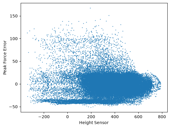
Each dot is one pixel, placed by its height and peak-force error. Separate clouds of dots would hint at distinct surface regions.

tracker.recording_start()

# --------- Block 2: Scatter plot between two channels ----------

name1, name2 = channel_names[0], channel_names[1]
img1, img2 = spice.data[:, :, 0], spice.data[:, :, 1]

fig, ax = plt.subplots()
ax.scatter(img1.ravel(), img2.ravel(), marker='o', s=.5)
ax.set_xlabel(name1)
ax.set_ylabel(name2)
plt.show()

tracker.recording_stop()

Choose the number of clusters

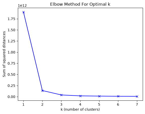
K-means needs the number of groups, k, in advance. The elbow method runs it for several k and plots how tightly pixels fit their groups; where the curve stops dropping steeply is a reasonable choice. This exploration uses scikit-learn directly and is not recorded in the history.

tracker.recording_start()

# --------- Block 3: Feature matrix + elbow method ----------

height, width, n_channels = spice.data.shape
features = spice.data.reshape(height * width, n_channels)
print(
    f'Number of pixels: {features.shape[0]}, '
    f'feature vector dimension: {features.shape[1]}'
)

K = range(1, 8)
inertias = []
for k in K:
    km = KMeans(n_clusters=k, n_init=10, random_state=0)
    km.fit(features)
    inertias.append(km.inertia_)

fig, ax = plt.subplots()
ax.plot(list(K), inertias, 'bx-')
ax.set_xlabel('k (number of clusters)')
ax.set_ylabel('Sum of squared distances')
ax.set_title('Elbow Method For Optimal k')
plt.show()

Number of pixels: 65536, feature vector dimension: 8

tracker.recording_stop()

Cluster the pixels

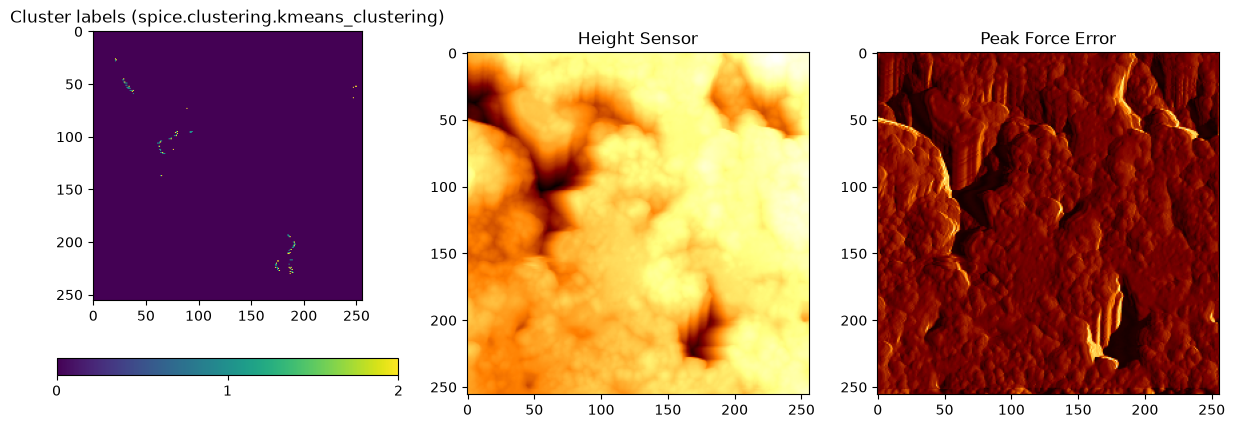
We use k = 3 with spice.clustering.kmeans_clustering(), which, unlike the other JuSPICE clustering methods, uses all channels of each pixel.

The channels are not rescaled. Since k-means compares distances, channels with large numerical spread (here DMTModulus, then Height Sensor) dominate the result.

tracker.recording_start()

# --------- Block 4: K-means clustering via spice.clustering ----------

km_spice = spice.clustering.kmeans_clustering(n_clusters=3, n_init=10, random_state=0)
print(f'km_spice.data.shape:  {km_spice.data.shape}')
print(f'clustering_method:    {km_spice.metadata["clustering_method"]}')
print(f'kmeans_inertia:       {km_spice.metadata["kmeans_inertia"]:.3e}')
print(f'cluster_centers.shape: {km_spice.extra["kmeans_cluster_centers"].shape}')

fig, ax = plt.subplots(1, 3, figsize=(15, 5))
im = ax[0].imshow(km_spice.data, cmap='viridis')
ax[0].set_title('Cluster labels (spice.clustering.kmeans_clustering)')
cbar = plt.colorbar(im, ax=ax[0], orientation='horizontal')
cbar.set_ticks(range(3))

ax[1].imshow(img1, cmap='afmhot')
ax[1].set_title(name1)

ax[2].imshow(img2, cmap='afmhot')
ax[2].set_title(name2)
plt.show()

km_spice.data.shape:  (256, 256)
clustering_method:    kmeans_clustering
kmeans_inertia:       3.888e+10
cluster_centers.shape: (3, 8)

tracker.recording_stop()

Save and review

We save the cluster map with its metadata and history script.

tracker.recording_start()

# --------- Block 5: Save ----------
# This folder holds several notebooks, so save_data()'s automatic
# notebook-name detection would be ambiguous when run outside a live
# Jupyter session (e.g. via nbconvert) — pass output_stem explicitly
# to always land on this notebook's own files. See
# docs/repository_structure.rst.
stem = 'io_afm2'
save_data(
    km_spice,
    output_stem=str(notebook_dir / stem),
)
print(f'Data:           {os.path.join(notebook_dir, stem + ".npy")}')
print(f'JSON sidecar:   {os.path.join(notebook_dir, stem + ".json")}')
print(f'History script: {os.path.join(notebook_dir, stem + "_history.py")}')

Data:           /Users/amir/GIT_repositories/juspice_pre_release/notebooks/io/io_afm2.npy
JSON sidecar:   /Users/amir/GIT_repositories/juspice_pre_release/notebooks/io/io_afm2.json
History script: /Users/amir/GIT_repositories/juspice_pre_release/notebooks/io/io_afm2_history.py

tracker.recording_stop()

The history lists every step as runnable code, including the clustering call.

tracker.recording_start()

# --------- Block 6: Inspect human-readable history ----------

readable_lines = km_spice.history.to_lines()
print('Reconstructed pipeline for this SPICEData object:')
print('\n'.join(readable_lines))

Reconstructed pipeline for this SPICEData object:
import juspice
spice = juspice.io.load_data('/Users/amir/GIT_repositories/juspice_pre_release/Sample_data/afm/example_file.spm')
km_spice = spice.clustering.kmeans_clustering(n_clusters=3, n_init=10, random_state=0)
juspice.io.save_data(spice)

tracker.recording_stop()