NMR : ILT without baseline artefact
[1]:
# This file is part of ILTpy examples.
# Author : Dr. Davis Thomas Daniel
# Last updated : 25.08.2025
This example shows steps to invert a NMR inversion recovery dataset without the baseline artefact.
It is recommended to familiarize yourself with the first example in the NMR section before continuing.
The data was acquired using sample of tetra-\(\mathrm{Li}_{7}\mathrm{SiPS}_{8}\) at a magic angle spinning frequency of 20 KHz and \(\nu_{31_{\mathrm{P}}}\) = 323 MHz.
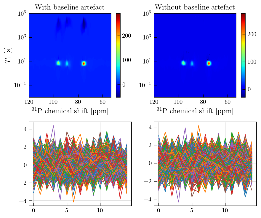
Inversion recovery curves may exhibit non-zero baselines, which may be interpreted by the algorithm as a slow relaxing component.
This artefact manifests in the obtained relaxation distribution as a negative peak with a long relaxation time constant (see comparison at the bottom and previous examples.)
This baseline artefact is avoided by adding an additional data point to the time trace and fitting the baseline as a single value.
In ILTpy, this can be achieved by setting the parameter ‘sb’ to True, however, this is currently only supported for 1D inversions.
This can be circumvented by doing 1D inversions of 2D data slices with ‘sb’ parameter set to True, as shown in this example.
Then, the data can be baseline corrected and a 2D inversion can be run again to obtain distributions without the baseline artefact.
Imports
The initial steps, loading and preparing data is the same as for any 2D inversion where only one dimension is inverted.
[2]:
# import iltpy
import iltpy as ilt

# other libraries for handling data, plotting
import numpy as np
import matplotlib.pyplot as plt
from tqdm import tqdm
plt.style.use('../../../examples/latex_style.mplstyle')
print(f"ILTpy version: {ilt.__version__}")
ILTpy version: 1.0.0
Data preparation
Load data from text files into numpy arrays
[3]:
# load data from text files into numpy arrays
lsps_data = np.loadtxt('../../../examples/NMR/inversion_recovery/data.txt')
lsps_vdlist = np.loadtxt('../../../examples/NMR/inversion_recovery/dim1.txt')
print(f'Original data size : {lsps_data.shape}')
Original data size : (15, 65536)
Data reduction
[4]:
# Reduce data by a moving mean
lsps_data_red = np.reshape(lsps_data,(15,1024,64))
lsps_data_red = np.squeeze(np.mean(lsps_data_red,axis=2))
print(f'Reduced data size : {lsps_data_red.shape}')
Reduced data size : (15, 1024)
The data consists of 15 recovery delays and for each delay, a spectrum of 65536 points.
To reduce computational demands of the inversion, the data is reduced.
The data was reduced to (15,1024) by moving mean.
Alternatively, number of points can be reduced by decreasing the sampling.
lsps_data_red = lsps_data[:,0:65536:65] # selects spectrum points with a spacing of 65 for each delay
Set noise variance to unity
[5]:
## Setting noise variance to unity

# To estimate noise, select a region with no signal
fig,ax = plt.subplots(figsize=(6,2.5),ncols=2)
ax[0].plot(lsps_data_red[-1])
ax[1].plot(lsps_data_red[-1][220:350])
ax[0].set_title('NMR spectrum')
ax[1].set_title('Noise region')
[5]:
Text(0.5, 1.0, 'Noise region')
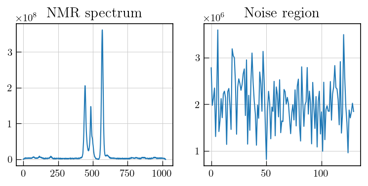
Note
The noise should be estimated from a region with random noise and no systematic features. In case of spectra with distorted baselines, the noise region can be obtained by doing an additional baseline correction for the corresponding region and then estimating the noise level.
[6]:
# and calculate the noise level
noise_lvl = np.std(lsps_data_red[-1][220:350])

# scale data with the noise_lvl
lsps_data_red = lsps_data_red/noise_lvl
ILTpy workflow
Load data
[7]:
lspsILT = ilt.iltload(data=lsps_data_red,t=lsps_vdlist)
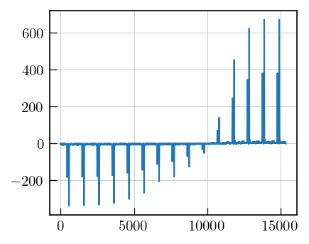
[8]:
# Plot the data
fig,ax = plt.subplots(figsize=(3,2.5))
a = ax.plot(lspsILT.data.flatten())
Initialization and inversion
1D inversions
Instead of inverting the 2D dataset, we extract individual slices of data and do multiple 1D inversions with ‘sb’ parameter set to True to remove the baseline artefact.
[9]:
tau = np.logspace(-2,5,100)
# get recovery traces for each point in the NMR spectrum
data1d_list = [lspsILT.data[:,j].copy() for j in range(lspsILT.data.shape[1])]

# initialize empty list for storing the results from 1D inversions
g1d_list = []
res1d_list = []

for i in tqdm(range(len(data1d_list))):
    lspsILT1d = ilt.iltload(data=data1d_list[i],t=lsps_vdlist)
    # set static baseline to True
    lspsILT1d.init(tau,kernel=ilt.Exponential(),parameters={'sb':True})
    # 1d inversion
    lspsILT1d.invert(verbose=-1)
    # store results
    g1d_list.append(lspsILT1d.g)
    res1d_list.append(lspsILT1d.residuals)
100%|██████████| 1024/1024 [01:46<00:00, 9.57it/s]
[10]:
# as an example, the distribution for the peak with maximum intensity is plotted below
idx = np.unravel_index(lspsILT.data.argmax(),lspsILT.data.shape)
fig,ax = plt.subplots(figsize=(3,2.5))
ax.semilogx(tau,-g1d_list[idx[1]][:-1]) #plotted with one point less, as the 'sb' feature adds an extra point to fit the baseline
_ = ax.set_xlabel(r'$T_{1}$'+' [s]')

Note
However, by inverting every point in the spectrum as a 1D data, we lose the improved resolution obtained as a result of regularizing the uninverted dimension.
We can use the distributions obtained from 1D inversions to remove the baseline artefact, as shown below.
Remove baseline artefact
Now, we invert again by correcting the baseline of data using the previously obtained distribution.
[11]:
# Baseline correct the data
data_bc = np.array(g1d_list)[:,-1] - lspsILT.data
[12]:
lspsILT_bc = ilt.iltload(data=data_bc,t=lsps_vdlist)
tau = np.logspace(-2,5,100)
lspsILT_bc.init(tau,kernel=ilt.Exponential())
lspsILT_bc.invert()
Starting iterations ...
100%|██████████| 100/100 [05:45<00:00, 3.46s/it]
Done.
For comparison, data without baseline correction is also inverted.
[13]:
tau = np.logspace(-2,5,100)
lspsILT.init(tau,kernel=ilt.Exponential())
lspsILT.invert()
Starting iterations ...
100%|██████████| 100/100 [05:37<00:00, 3.37s/it]
Done.
Plot the results
Note
The plots below compare the data with and without the baseline artefact.
In the data without addtional baseline correction as demonstrated above, ngative features with long relaxation time constants are observed.
In both cases, residuals obtained are random with no systematic features.
[14]:
# load the chemical shift axis for plotting
ppm_axis = np.loadtxt('../../../examples/NMR/inversion_recovery/chemical_shift_axis.txt')
ppm_axis = np.reshape(ppm_axis,(1024,64))
ppm_axis = np.mean(ppm_axis,axis=1)


fig,ax = plt.subplots(ncols=2,nrows=2,figsize=(6,5))

g = ax[0,0].pcolor(ppm_axis[300:700],lspsILT.tau[0].flatten(),np.negative(lspsILT.g[:,300:700]),cmap='jet')
ax[0,0].set_yscale('log')
ax[0,0].set_ylabel(r'$T_{1}$'+' [s]')
ax[0,0].set_xlabel(r'$^{31}\mathrm{P}$'+' chemical shift [ppm]')
ax[0,0].invert_xaxis()
fig.colorbar(g,ax=ax[0,0])
ax[0,0].grid()
ax[0,0].set_title('With baseline artefact',fontsize=12)


g_bc = ax[0,1].pcolor(ppm_axis[300:700],lspsILT_bc.tau[0].flatten(),lspsILT_bc.g[:,300:700],cmap='jet')
ax[0,1].set_yscale('log')
ax[0,1].set_xlabel(r'$^{31}\mathrm{P}$'+' chemical shift [ppm]')
ax[0,1].invert_xaxis()
fig.colorbar(g_bc,ax=ax[0,1])
ax[0,1].grid()
ax[0,1].set_title('Without baseline artefact',fontsize=12)

ax[1,0].plot(lspsILT.residuals)
_ = ax[1,1].plot(lspsILT_bc.residuals)

fig.tight_layout()