EPR : Pronounced ESEEM case
[1]:
# This file is part of ILTpy examples.
# Author : Dr. Davis Thomas Daniel
# Last updated : 16.02.2026
This example shows steps to invert an EPR echo decay dataset in the presence of pronounced electron spin echo envelope modulations.
It is recommended to familiarize yourself with the first example in the EPR section before continuing.
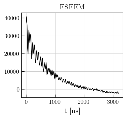
Laplace inversion of electron spin echo decay data in the presence of oscillations on the spin echo decay curve due to electron spin echo envelope modulation (ESEEM) sometimes leads to overfitting of the oscillations at short echo times.
This example shows how to circumvent this overfitting by using the amplitude of oscillations as a noise estimate.
Importing iltpy and loading data
[2]:
# import iltpy
import iltpy as ilt

# other libraries for handling data, plotting
import numpy as np
import matplotlib.pyplot as plt
import matplotlib.gridspec as gridspec
from copy import deepcopy
print(f"ILTpy version: {ilt.__version__}")
ILTpy version: 1.1.0
[3]:
# Load data
eseem_data = np.genfromtxt('../../../examples/EPR/eseem/eseem.csv',delimiter=',')
eseemILT = ilt.iltload(data=eseem_data[:,1],t=eseem_data[:,0]) # second column is the data (or echo intensity) and first column is the tau delays
[4]:
# Plot the raw data
fig,ax = plt.subplots(figsize=(4,3.5))
ax.plot(eseemILT.t[0].flatten()[0:200],eseemILT.data[0:200],'k')
plt.xlabel('t [ns]')
a1 = plt.title('ESEEM',size=12)
Data preparation
[5]:
# Data preparation, consult previous examples for details

x,y = eseemILT.t[0][924:],eseemILT.data[924:]
m,b = np.polyfit(x, y, 1)
noise_lvl = np.std(eseemILT.data[924:]-m*x+b)

eseemILT.data = eseemILT.data/noise_lvl
Initialization and inversion
[7]:
tau = np.logspace(0,6,121)
eseemILT.init(tau,kernel=ilt.Gaussian())
eseemILT.invert()
Starting iterations ...
100%|██████████| 100/100 [00:00<00:00, 489.18it/s, Convergence=2.67e-02]
Done.
[9]:
# Plot the raw data
fig,ax = plt.subplots(figsize=(5,3.5))
# data and fit
ax.plot(eseemILT.t[0].flatten()[0:200], eseemILT.data[0:200], color='#1f77b4', label='Exp.', linewidth=2)
ax.plot(eseemILT.t[0].flatten()[0:200], eseemILT.fit[0:200], color='#ff7f0e', linestyle='dashed', label='Fit')
ax.set_xlabel('t [ns]')
ax.legend()
a1 = ax.set_title('Data and fit')
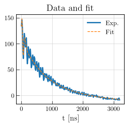
Note
Laplace inversion of electron spin echo decay data in the presence of oscillations on the spin echo decay curve due to electron spin echo envelope modulation (ESEEM) sometimes leads to overfitting of the oscillations at short echo times (see the figure above).
This can be circumvented by employing a weighted Laplace inversion by providing ‘sigma’ as a parameter during inversion.
sigma is a guess of the non-uniform amplitude of the ESEEM oscillations as a noise estimate, thereby treating ESEEM modulations as noise on the relaxation curve.
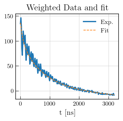
Weighted inversion
[10]:
## use residuals from previous inversion as noise estimate
from scipy.ndimage import uniform_filter1d
# window size for movmean selected based on period of ESEEM oscillations
sigma = uniform_filter1d(np.abs(eseemILT.residuals),8)

# make a copy of the previous IltData instance
eseemILT_weighted  = deepcopy(eseemILT)
# same parameters as before, but with sigma defined
tau = np.logspace(0,6,121)
eseemILT_weighted.init(tau,kernel=ilt.Gaussian(),sigma=sigma,parameters={'sb':True})
eseemILT_weighted.invert()
Starting iterations ...
28%|██▊ | 28/100 [00:00<00:00, 439.31it/s, Convergence=8.71e-07]
Convergence limit reached at iteration 28.
Done.
[12]:
# Plot the raw data
fig,ax = plt.subplots(figsize=(5,3.5))
# data and fit
ax.plot(eseemILT_weighted.t[0].flatten()[0:200], eseemILT_weighted.data[0:200], color='#1f77b4', label='Exp.', linewidth=2)
ax.plot(eseemILT_weighted.t[0].flatten()[0:200], eseemILT_weighted.fit[0:200], color='#ff7f0e', linestyle='dashed', label='Fit')
ax.set_xlabel('t [ns]')
ax.legend()
a1 = ax.set_title('Weighted Data and fit')
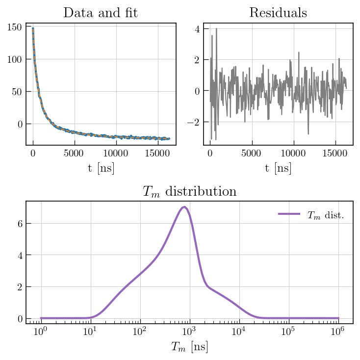
[13]:
fig = plt.figure(figsize=(7, 7))
gs = gridspec.GridSpec(2, 2, width_ratios=[1, 1])

ax0 = fig.add_subplot(gs[0])
ax1 = fig.add_subplot(gs[1])
ax2 = fig.add_subplot(gs[1,0:])

# data and fit
ax0.plot(eseemILT_weighted.t[0].flatten(), eseemILT_weighted.data, color='#1f77b4', label='Exp.', linewidth=2)
ax0.plot(eseemILT_weighted.t[0].flatten(), eseemILT_weighted.fit, color='#ff7f0e', linestyle='dashed', label='Fit')
ax0.set_xlabel('t [ns]')
ax0.set_title('Data and fit')

# residuals
ax1.plot(eseemILT_weighted.t[0].flatten(), eseemILT_weighted.residuals, color='#7f7f7f')
ax1.set_title('Residuals')
ax1.set_xlabel('t [ns]')

# Distribution
ax2.semilogx(eseemILT_weighted.tau[0].flatten(), eseemILT_weighted.g[:-1], color='#9467bd', label=r'$T_m$'+' dist. (weighted)',linewidth=2)

ax2.set_title(r'$T_m$'+' distribution')
ax2.set_xlabel(r'$T_m$'+' [ns]')
ax2.legend()

plt.tight_layout()
plt.show()
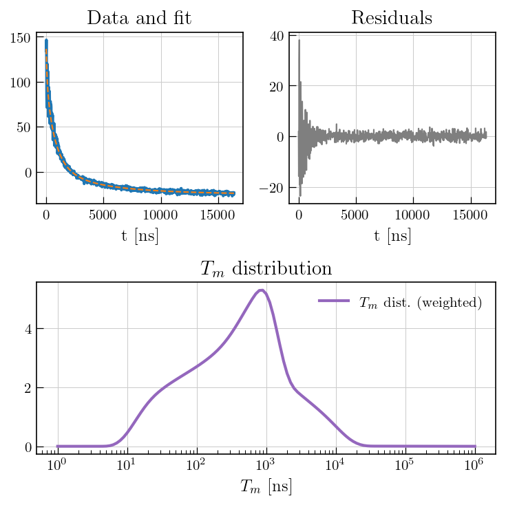
Note
While the weighted inversion \(^1\) seems to prevent the overfitting, ESEEM interactions may cause a strongly damped initial echo decay that might lead to spurious relaxation modes with some kernels. To avoid overinterpretation of data, such artificial modes must to be distinguished from real relaxation modes, e.g. by multi-frequency EPR. Moreover, modulation interference of ESEEM combination frequencies significantly affects initial echo decay, which might be mistaken as relaxation of the unmodulated part of the decay time trace.\(^2\) Therefore, quantitativity of such data must be assessed individually for a particular type of sample in case of severe ESEEM oscillations on the Hahn echo decay.
Merz et al. Molecules, 2021, 26, 6690.
Kasumaj et al. Journal of Magnetic Resonance, 2012, 223, 187–197.
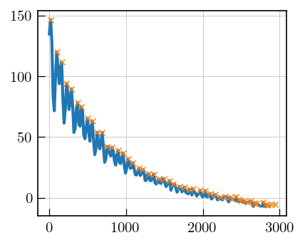
Alternative approach for ESEEM data
In this approach, points are picked on decay and the picked points are fitted.
[14]:
from scipy.signal import find_peaks
[15]:
# make a copy of the previous IltData instance
eseemILT_alt  = deepcopy(eseemILT)

peaks,_ = find_peaks(eseemILT_alt.data)

# Plot the raw data
fig,ax = plt.subplots(figsize=(5,3.5))
# data and fit
ax.plot(eseemILT_alt.t[0].flatten()[0:180],eseemILT_alt.data[0:180],
        color='#1f77b4', label='Exp.', linewidth=2)
_=ax.plot(eseemILT_alt.t[0].flatten()[peaks][0:50],eseemILT_alt.data[peaks][0:50].flatten(),
        color='#ff7f0e', marker='x', label='Fit',linewidth=0)
[16]:
## set only the decay curve as data
eseemILT_alt.data = eseemILT_alt.data[peaks]
eseemILT_alt.t[0] = eseemILT_alt.t[0].flatten()[peaks]
[17]:
## initialize and invert
tau = np.logspace(0,6,121)
eseemILT_alt.init(tau,kernel=ilt.Gaussian(),parameters={'sb':True})
eseemILT_alt.invert()
Starting iterations ...
28%|██▊ | 28/100 [00:00<00:00, 457.28it/s, Convergence=7.52e-07]
Convergence limit reached at iteration 28.
Done.
[18]:
fig = plt.figure(figsize=(7, 7))
gs = gridspec.GridSpec(2, 2, width_ratios=[1, 1])

ax0 = fig.add_subplot(gs[0])
ax1 = fig.add_subplot(gs[1])
ax2 = fig.add_subplot(gs[1,0:])

# data and fit
ax0.plot(eseemILT_alt.t[0].flatten(), eseemILT_alt.data, color='#1f77b4', label='Exp.', linewidth=2)
ax0.plot(eseemILT_alt.t[0].flatten(), eseemILT_alt.fit, color='#ff7f0e', linestyle='dashed', label='Fit')
ax0.set_xlabel('t [ns]')
ax0.set_title('Data and fit')

# residuals
ax1.plot(eseemILT_alt.t[0].flatten(), eseemILT_alt.residuals, color='#7f7f7f')
ax1.set_title('Residuals')
ax1.set_xlabel('t [ns]')

# Distribution
ax2.semilogx(eseemILT_alt.tau[0].flatten(), eseemILT_alt.g[:-1], color='#9467bd', label=r'$T_m$'+' dist.',linewidth=2)

ax2.set_title(r'$T_m$'+' distribution')
ax2.set_xlabel(r'$T_m$'+' [ns]')
ax2.legend()

plt.tight_layout()
plt.show()