Influence of the number of data points on inversion
[ ]:
# This file is part of ILTpy examples.
# Author : Dr. Davis Thomas Daniel
# Last updated : 18.08.2025
This example tests the influence of the number of data points on the inversion results.
For this example, we use a NMR CPMG data set and vary the number of points in second dimension (spectrum) which is not inverted but regularized.
This example was run on machine running Ubuntu 22.04.5 and python was restricted to use only 4 CPU cores.
Imports
[1]:
# import iltpy
import iltpy as ilt
print(ilt.__version__)

# other libraries for handling data, plotting
import numpy as np
import matplotlib.pyplot as plt

# for monitoring resource usage
import subprocess
import time
import os
1.0b9
For monitoring the resource usage during inversion, a separate python script is made which is saved as monitor_resources.py
import psutil
import os

LOG_FILE = "resource_log.txt"
PID_TO_MONITOR = int(os.environ.get("TARGET_PID", 0))

def monitor(pid):
    process = psutil.Process(pid)
    with open(LOG_FILE, "a") as f:
        while True:
            try:
                cpu = process.cpu_percent(interval=1)
                mem = process.memory_info().rss / 1024**2  # MB
                f.write(f"{cpu:.2f}, {mem:.2f}\n")
                f.flush()
            except psutil.NoSuchProcess:
                break

if PID_TO_MONITOR:
    monitor(PID_TO_MONITOR)
else:
    print("No PID provided to monitor.")
[5]:
# start monitoring
monitor_proc = subprocess.Popen(
    ["python", "monitor_resources.py"],
    env={**os.environ, "TARGET_PID": str(os.getpid())}
)

# another help function to log data shapes to the same file
def log_message(msg):
    with open("resource_log.txt", 'a') as f:
        timestamp = time.strftime('%Y-%m-%d %H:%M:%S')
        f.write(f"{timestamp}, {msg}\n")
Data preparation
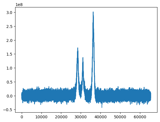
The data consists of 8 echo delays and for each delay, a spectrum of 65536 points.
We use this data set to create multiple data sets of different sizes in the second dimension (spectrum)
Load data from text files into numpy arrays
[3]:
cpmg_data = np.loadtxt('../../../examples/NMR/CPMG/data.txt') # spectra
cpmg_delays = np.loadtxt('../../../examples/NMR/CPMG/dim1.txt') #  cpmg echo delays

print(f"Original data size : {cpmg_data.shape}")
Original data size : (8, 65536)
[4]:
# first spectrum
fig,ax = plt.subplots()
_=ax.plot(cpmg_data[0])
Set noise variance to unity
[5]:
cpmg_data = cpmg_data/np.std(cpmg_data[0,0:1000])
Data reduction
[6]:
# Reduce data by a moving mean or by reducing the sampling

cpmg_red_32768 = cpmg_data[:,0::2] # 8x32768
cpmg_red_16384 = cpmg_data[:,0::4] # 8x16384
cpmg_red_8192 = cpmg_data[:,0::8] # 8x8192
cpmg_red_4096 = cpmg_data[:,0::16] # 8x4096
cpmg_red_2048 = cpmg_data[:,0::32] # 8x2048
cpmg_red_1024 = cpmg_data[:,0::64] # 8x1024
cpmg_red_512 = cpmg_data[:,0::128] # 8x512
Initialization and inversion
[9]:
tau = np.logspace(-4,1,35) # tau array with 35 points ranging from 10^-4 to 10^1
[10]:
cpu_times = []
[10]:
# 512 points
start = time.process_time()
log_message(f"Inversion with data shape : {cpmg_red_512.shape}")
ilt_512 = ilt.iltload(data=cpmg_red_512,t=cpmg_delays)
ilt_512.init(tau=tau,kernel=ilt.Exponential())
ilt_512.invert()
log_message("####")
end = time.process_time()
cpu_times.append(end-start)
print(f"CPU time taken : {end-start} s.")

# 1024 points
start = time.process_time()
log_message(f"Inversion with data shape : {cpmg_red_1024.shape}")
ilt_1024 = ilt.iltload(data=cpmg_red_1024,t=cpmg_delays)
ilt_1024.init(tau=tau,kernel=ilt.Exponential())
ilt_1024.invert()
log_message("####")
end = time.process_time()
cpu_times.append(end-start)
print(f"CPU time taken : {end-start} s.")

# 2048 points
start = time.process_time()
log_message(f"Inversion with data shape : {cpmg_red_2048.shape}")
ilt_2048 = ilt.iltload(data=cpmg_red_2048,t=cpmg_delays)
ilt_2048.init(tau=tau,kernel=ilt.Exponential())
ilt_2048.invert()
log_message("####")
end = time.process_time()
cpu_times.append(end-start)
print(f"CPU time taken : {end-start} s.")

# 4096 points
start = time.process_time()
log_message(f"Inversion with data shape : {cpmg_red_4096.shape}")
ilt_4096 = ilt.iltload(data=cpmg_red_4096,t=cpmg_delays)
ilt_4096.init(tau=tau,kernel=ilt.Exponential())
ilt_4096.invert()
log_message("####")
end = time.process_time()
cpu_times.append(end-start)
print(f"CPU time taken : {end-start} s.")

# 8192 points
start = time.process_time()
log_message(f"Inversion with data shape : {cpmg_red_8192.shape}")
ilt_8192 = ilt.iltload(data=cpmg_red_8192,t=cpmg_delays)
ilt_8192.init(tau=tau,kernel=ilt.Exponential())
ilt_8192.invert()
log_message("####")
end = time.process_time()
cpu_times.append(end-start)
print(f"CPU time taken : {end-start} s.")

# 16384 points
start = time.process_time()
log_message(f"Inversion with data shape : {cpmg_red_16384.shape}")
ilt_16384 = ilt.iltload(data=cpmg_red_16384,t=cpmg_delays)
ilt_16384.init(tau=tau,kernel=ilt.Exponential())
ilt_16384.invert()
log_message("####")
end = time.process_time()
cpu_times.append(end-start)
print(f"CPU time taken : {end-start} s.")

# 32768 points
start = time.process_time()
log_message(f"Inversion with data shape : {cpmg_red_32768.shape}")
ilt_32768 = ilt.iltload(data=cpmg_red_32768,t=cpmg_delays)
ilt_32768.init(tau=tau,kernel=ilt.Exponential())
ilt_32768.invert()
log_message("####")
end = time.process_time()
cpu_times.append(end-start)
print(f"CPU time taken : {end-start} s.")

monitor_proc.terminate()
Starting iterations ...
100%|██████████████████████████████████████████████████████████████████████████████████████████████████████████████████████████████████████████████████████████████████████████████████████████| 100/100 [00:34<00:00, 2.88it/s]
Done.
CPU time taken : 43.053515448 s.
Starting iterations ...
100%|██████████████████████████████████████████████████████████████████████████████████████████████████████████████████████████████████████████████████████████████████████████████████████████| 100/100 [00:54<00:00, 1.85it/s]
Done.
CPU time taken : 55.037861299 s.
Starting iterations ...
100%|██████████████████████████████████████████████████████████████████████████████████████████████████████████████████████████████████████████████████████████████████████████████████████████| 100/100 [01:29<00:00, 1.12it/s]
Done.
CPU time taken : 90.346509413 s.
Starting iterations ...
100%|██████████████████████████████████████████████████████████████████████████████████████████████████████████████████████████████████████████████████████████████████████████████████████████| 100/100 [02:46<00:00, 1.67s/it]
Done.
CPU time taken : 164.95304677599998 s.
Starting iterations ...
100%|██████████████████████████████████████████████████████████████████████████████████████████████████████████████████████████████████████████████████████████████████████████████████████████| 100/100 [05:29<00:00, 3.30s/it]
Done.
CPU time taken : 324.903184168 s.
Starting iterations ...
100%|██████████████████████████████████████████████████████████████████████████████████████████████████████████████████████████████████████████████████████████████████████████████████████████| 100/100 [10:37<00:00, 6.37s/it]
Done.
CPU time taken : 636.1182191280001 s.
Starting iterations ...
100%|██████████████████████████████████████████████████████████████████████████████████████████████████████████████████████████████████████████████████████████████████████████████████████████| 100/100 [20:58<00:00, 12.59s/it]
Done.
CPU time taken : 1261.121670039 s.
[11]:
ilt_list = [ilt_512,ilt_1024,ilt_2048,ilt_4096,ilt_8192,ilt_16384,ilt_32768]
data_shape_list = [2**i for i in range(9,16)]

for iltdata, shape in zip(ilt_list,data_shape_list):
    print(f"Shape A: {iltdata.W.shape} and B: {iltdata.Y.shape} in Ax=B. Data shape: (8,{shape}), Tau size: {iltdata.tau[0].size}, Inversion time : {iltdata.inversion_time:.1f}s")
    np.save(f"g_{shape}.npy",iltdata.g)
    np.save(f"residuals_{shape}.npy",iltdata.residuals)
    np.save(f"fit_{shape}.npy",iltdata.fit)
Shape A: (17920, 17920) and B: (17920, 1) in Ax=B. Data shape: (8,512), Tau size: 35, Inversion time : 34.7s
Shape A: (35840, 35840) and B: (35840, 1) in Ax=B. Data shape: (8,1024), Tau size: 35, Inversion time : 54.1s
Shape A: (71680, 71680) and B: (71680, 1) in Ax=B. Data shape: (8,2048), Tau size: 35, Inversion time : 89.3s
Shape A: (143360, 143360) and B: (143360, 1) in Ax=B. Data shape: (8,4096), Tau size: 35, Inversion time : 166.6s
Shape A: (286720, 286720) and B: (286720, 1) in Ax=B. Data shape: (8,8192), Tau size: 35, Inversion time : 329.5s
Shape A: (573440, 573440) and B: (573440, 1) in Ax=B. Data shape: (8,16384), Tau size: 35, Inversion time : 637.1s
Shape A: (1146880, 1146880) and B: (1146880, 1) in Ax=B. Data shape: (8,32768), Tau size: 35, Inversion time : 1259.0s
Resource usage as a function of matrix size
[17]:
# parse the resource usage log

def parse_resource_log(filename):
    cpu_blocks, mem_blocks, shape_labels = [], [], []
    cpu, mem, shape = [], [], None

    with open(filename) as f:
        for line in f:
            if "Inversion with data shape" in line:
                if shape:
                    cpu_blocks.append(cpu)
                    mem_blocks.append(mem)
                    shape_labels.append(shape)
                cpu, mem = [], []
                shape = line.split(":")[-1].strip()
            else:
                try:
                    parts = line.strip().split(", ")
                    cpu.append(float(parts[0]))
                    mem.append(float(parts[1]))
                except:
                    continue

    if shape:
        cpu_blocks.append(cpu)
        mem_blocks.append(mem)
        shape_labels.append(shape)

    return cpu_blocks,mem_blocks,shape_labels
[ ]:
# Save the generated resource_log.txt file as resource_log_4core.txt

cpu_blocks_4core,mem_blocks_4core,_ = parse_resource_log("resource_log_4core.txt")
cpu_blocks_4core_mean = [np.mean(cpu_usage) for cpu_usage in cpu_blocks_4core]
mem_blocks_4core_mean = [np.mean(mem_usage) for mem_usage in mem_blocks_4core]
[57]:
np.mean(cpu_blocks_4core_mean) # with alt_g = 0, computation runs on single core.
[57]:
np.float64(102.6709257661353)
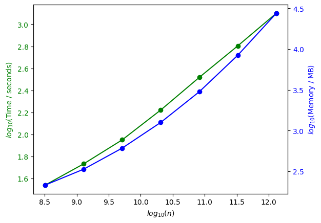
Memory usage and inversion time
[ ]:
matrix_sizes = (
    np.array([17920, 35840, 71680, 143360, 286720, 573440, 1146880]) ** 2
)  # total number of elements
log10_x = np.log10(matrix_sizes)

inversion_time_list = [34.7, 54.1, 89.3, 166.6, 329.5, 637.1, 1259.0]  # in seconds
log10_time = np.log10(inversion_time_list)

log10_memory = np.log10(mem_blocks_4core_mean)

fig, ax1 = plt.subplots()
ax1.plot(log10_x, log10_time, "-og", label="Time")
ax2 = ax1.twinx()
ax2.plot(log10_x, log10_memory, "-ob", label="Memory")

ax1.set_xlabel(r"$log_{10}(n)$")
ax1.set_ylabel(r"$log_{10}$" + "(Time / seconds)", color="g")

ax2.set_xlabel(r"$log_{10}(n)$")
ax2.set_ylabel(r"$log_{10}$" + "(Memory / MB)", color="b")

ax1.tick_params(axis="y", labelcolor="g")
ax2.tick_params(axis="y", labelcolor="b")
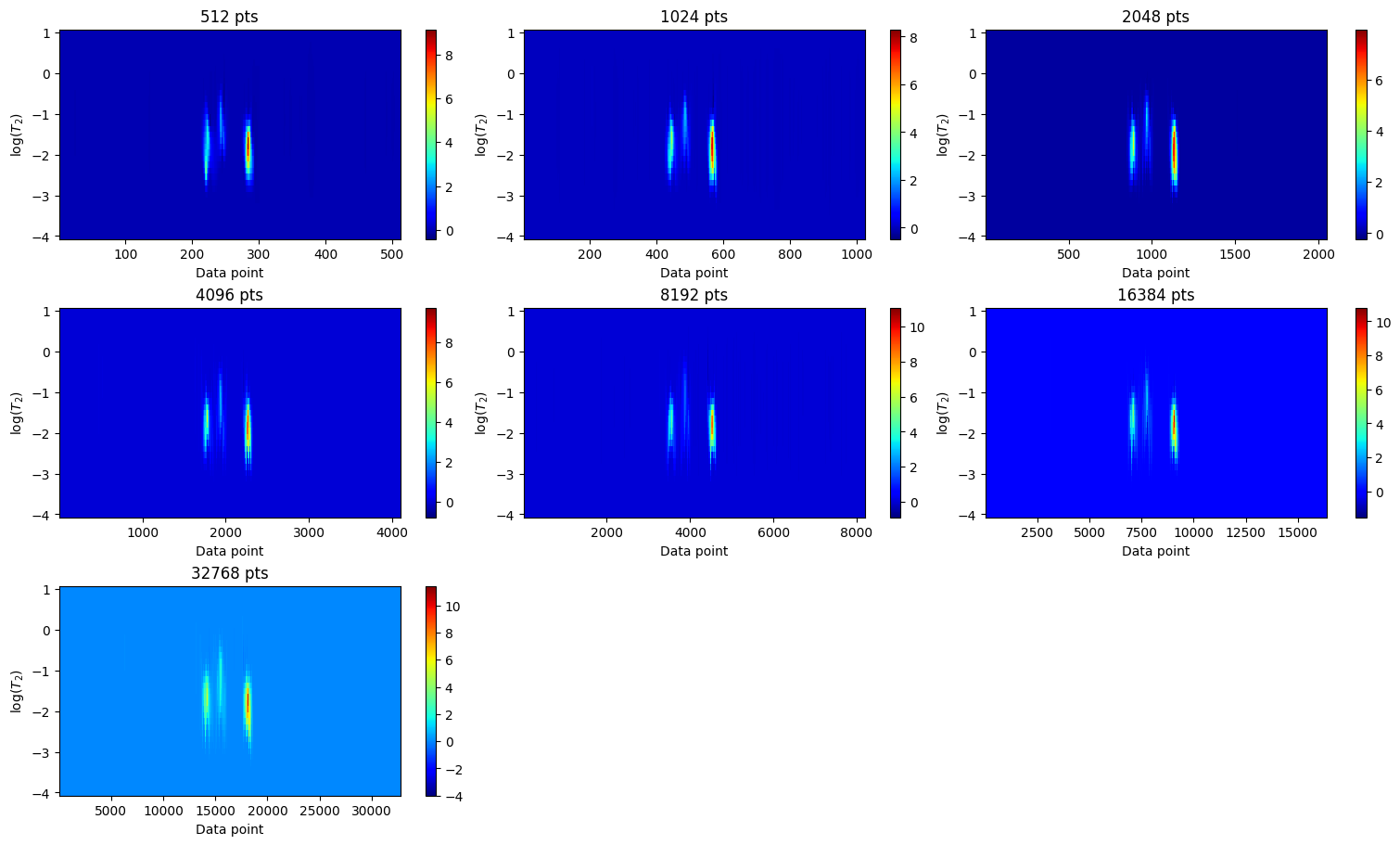
Relaxation distribution
[22]:
ilt_list = [ilt_512, ilt_1024, ilt_2048, ilt_4096, ilt_8192, ilt_16384, ilt_32768]
fig, axes = plt.subplots(3, 3, figsize=(15, 9), constrained_layout=True)
axes = axes.flatten()

for ax, iltdata in zip(axes, ilt_list):
    t = iltdata.t[1].flatten()
    tau = np.log10(iltdata.tau[0].flatten())
    g = iltdata.g
    c = ax.pcolor(t, tau, g, shading='auto',cmap="jet")
    ax.set_title(f"{g.shape[1]} pts")
    ax.set_xlabel("Data point")
    ax.set_ylabel(r"log($T_{2}$)")
    fig.colorbar(c, ax=ax)


for ax in axes[len(ilt_list):]:
    ax.remove()

plt.show()

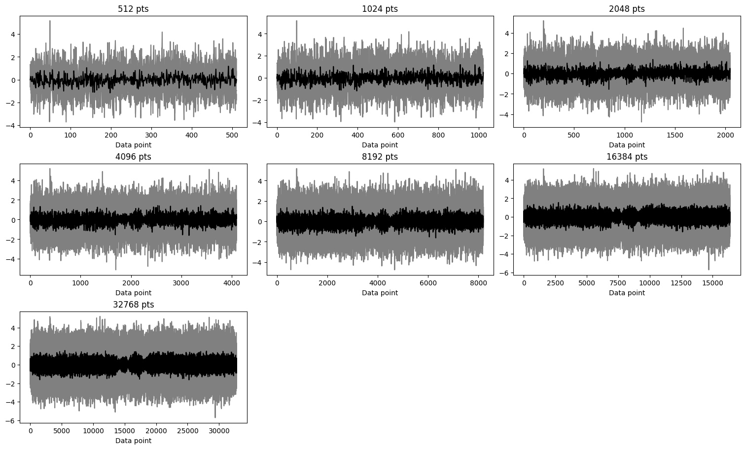
Residuals
[25]:
fig, axes = plt.subplots(3, 3, figsize=(15, 9), constrained_layout=True)
axes = axes.flatten()

for ax, iltdata in zip(axes, ilt_list):

    res = iltdata.residuals
    ax.plot(res.T,color='grey')
    ax.plot(res.mean(axis=0),'k')
    ax.set_title(f"{res.shape[1]} pts")
    ax.set_xlabel("Data point")

for ax in axes[len(ilt_list):]:
    ax.remove()

plt.show()

In the case of this dataset, for all the data sizes, the distributions are similar and the residuals show random noise without any systematic features.
Qualitatively, the number of data points along the spectral dimension (i.e., the dimension that is regularized but not inverted) should be sufficient to ensure that each resonance peak is sampled with greater density than its full width at half maximum (FWHM).
Note that, we used the same input sampling vector in the uninverted dimension (with unity spacing by default) for all different data sizes. Depending on sample density, this should be adjusted for different data sets.
Appendix : Inversion using Sparse Cholesky Factorisation
By default, ILTpy uses scipy’s spsolve to solve equations of type Ax=B, which in turn uses LU factorisation to solve.
Using sparse Cholesky factorisation, the computation time can be reduced.
This requires the installation of another library, scikit-sparse.
This section of the example was run on a machine with 8 core Apple M1 processor and 16 GB of memory.
Define a solver function to use with ILTpy
[7]:
from sksparse.cholmod import cholesky

def skit_solver(A,b):
    factor = cholesky(A)
    return factor(b).flatten()
Initialize and invert using custom solver
[8]:
# we use the data and functions which are already defined for the main example.
[9]:
tau = np.logspace(-4,1,35) # tau array with 35 points ranging from 10^-4 to 10^1
[10]:
# 512 points
ilt_512 = ilt.iltload(data=cpmg_red_512,t=cpmg_delays)
ilt_512.init(tau=tau,kernel=ilt.Exponential())
ilt_512.invert(solver=skit_solver) # specify the solver

# 1024 points
ilt_1024 = ilt.iltload(data=cpmg_red_1024,t=cpmg_delays)
ilt_1024.init(tau=tau,kernel=ilt.Exponential())
ilt_1024.invert(solver=skit_solver) # specify the solver

# 2048 points
ilt_2048 = ilt.iltload(data=cpmg_red_2048,t=cpmg_delays)
ilt_2048.init(tau=tau,kernel=ilt.Exponential())
ilt_2048.invert(solver=skit_solver) # specify the solver

# 4096 points
ilt_4096 = ilt.iltload(data=cpmg_red_4096,t=cpmg_delays)
ilt_4096.init(tau=tau,kernel=ilt.Exponential())
ilt_4096.invert(solver=skit_solver) # specify the solver

# 8192 points
ilt_8192 = ilt.iltload(data=cpmg_red_8192,t=cpmg_delays)
ilt_8192.init(tau=tau,kernel=ilt.Exponential())
ilt_8192.invert(solver=skit_solver) # specify the solver

# 16384 points
ilt_16384 = ilt.iltload(data=cpmg_red_16384,t=cpmg_delays)
ilt_16384.init(tau=tau,kernel=ilt.Exponential())
ilt_16384.invert(solver=skit_solver) # specify the solver

# 32768 points
ilt_32768 = ilt.iltload(data=cpmg_red_32768,t=cpmg_delays)
ilt_32768.init(tau=tau,kernel=ilt.Exponential())
ilt_32768.invert(solver=skit_solver) # specify the solver
Starting iterations ...
100%|██████████| 100/100 [00:07<00:00, 13.69it/s]
Done.
Starting iterations ...
100%|██████████| 100/100 [00:14<00:00, 7.06it/s]
Done.
Starting iterations ...
100%|██████████| 100/100 [00:28<00:00, 3.52it/s]
Done.
Starting iterations ...
100%|██████████| 100/100 [00:56<00:00, 1.77it/s]
Done.
Starting iterations ...
100%|██████████| 100/100 [01:56<00:00, 1.17s/it]
Done.
Starting iterations ...
100%|██████████| 100/100 [03:44<00:00, 2.24s/it]
Done.
Starting iterations ...
100%|██████████| 100/100 [08:01<00:00, 4.81s/it]
Done.
[11]:
from copy import deepcopy

# 512 points
ilt_512lu = deepcopy(ilt_512)
ilt_512lu.invert() # repeat with default solver

# 1024 points
ilt_1024lu = deepcopy(ilt_1024)
ilt_1024lu.invert() # repeat with default solver

# 2048 points
ilt_2048lu = deepcopy(ilt_2048)
ilt_2048lu.invert() # repeat with default solver

# 4096 points
ilt_4096lu = deepcopy(ilt_4096)
ilt_4096lu.invert() # repeat with default solver

# 8192 points
ilt_8192lu = deepcopy(ilt_8192)
ilt_8192lu.invert() # repeat with default solver

# 16384 points
ilt_16384lu = deepcopy(ilt_16384)
ilt_16384lu.invert() # repeat with default solver

# 32768 points
ilt_32768lu = deepcopy(ilt_32768)
ilt_32768lu.invert() # repeat with default solver
Starting iterations ...
100%|██████████| 100/100 [00:11<00:00, 8.58it/s]
Done.
Starting iterations ...
100%|██████████| 100/100 [00:24<00:00, 4.05it/s]
Done.
Starting iterations ...
100%|██████████| 100/100 [00:50<00:00, 1.98it/s]
Done.
Starting iterations ...
100%|██████████| 100/100 [01:44<00:00, 1.05s/it]
Done.
Starting iterations ...
100%|██████████| 100/100 [03:27<00:00, 2.08s/it]
Done.
Starting iterations ...
100%|██████████| 100/100 [07:05<00:00, 4.25s/it]
Done.
Starting iterations ...
100%|██████████| 100/100 [14:50<00:00, 8.90s/it]
Done.
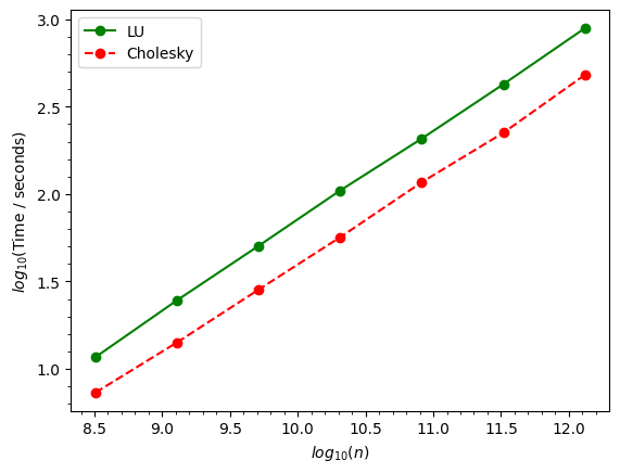
Compare inversion time
[ ]:
# we compare inversion time between the LU and cholkesky factorisation.

matrix_sizes = np.array([17920,35840,71680,143360,286720,573440,1146880])**2 # total number of elements
log10_x = np.log10(matrix_sizes)
data_list_lu = [ilt_512lu,ilt_1024lu,ilt_2048lu,ilt_4096lu,ilt_8192lu,ilt_16384lu,ilt_32768lu]
data_list_chol = [ilt_512,ilt_1024,ilt_2048,ilt_4096,ilt_8192,ilt_16384,ilt_32768]

inversion_time_list_skitsparse = [i.inversion_time for i in data_list_chol] # in seconds, from cholesky factorisaition
inversion_time_list = [i.inversion_time for i in data_list_lu] # in seconds, from LU factorisarion
log10_time_skitsparse = np.log10(inversion_time_list_skitsparse)
log10_time = np.log10(inversion_time_list)


fig,ax = plt.subplots()
ax.plot(log10_x,log10_time,'-og',label="LU")
ax.plot(log10_x,log10_time_skitsparse,'--or',label="Cholesky")
ax.set_xlabel(r"$log_{10}(n)$")
ax.set_ylabel(r"$log_{10}$"+"(Time / seconds)")
ax.minorticks_on()
_=ax.legend()
132.72085714285714
244.96085714285715
Relaxation distribution
[19]:
ilt_list = [ilt_512, ilt_1024, ilt_2048, ilt_4096, ilt_8192, ilt_16384, ilt_32768]
fig, axes = plt.subplots(3, 3, figsize=(15, 9), constrained_layout=True)
axes = axes.flatten()

for ax, iltdata in zip(axes, ilt_list):
    t = iltdata.t[1].flatten()
    tau = np.log10(iltdata.tau[0].flatten())
    g = iltdata.g
    c = ax.pcolor(t, tau, g, shading='auto',cmap="jet")
    ax.set_title(f"{g.shape[1]} pts")
    ax.set_xlabel("Data point")
    ax.set_ylabel(r"log($T_{2}$)")
    fig.colorbar(c, ax=ax)

for ax in axes[len(ilt_list):]:
    ax.remove()

plt.show()
Residuals
[30]:
fig, axes = plt.subplots(3, 3, figsize=(15, 9), constrained_layout=True)
axes = axes.flatten()

for ax, iltdata in zip(axes, ilt_list):

    res = iltdata.residuals
    ax.plot(res.T,color='grey')
    ax.plot(res.mean(axis=0),'k')
    ax.set_title(f"{res.shape[1]} pts")
    ax.set_xlabel("Data point")

for ax in axes[len(ilt_list):]:
    ax.remove()

plt.show()
The results remain the same, irrespective of the solver used.