Using other sparse solvers

# This file is part of IltPy examples.
# Author : Dr. Davis Thomas Daniel
# Last updated : 18.05.2025

• During inversion and with default alt_g=0, IltPy solves an equation of the form : Ax=B where A is sparse matrix of type scipy.sparse._csc.csc_matrix (Compressed Sparse Column matrix) and B is of type np.ndarray.

• By default, scipy’s spsolve(permc_spec='NATURAL',use_umfpack=True) or solve is used for solving, depending on kernel sparsity. In the sparse format, natural ordering is used to permute the columns of the matrix for sparsity preservation and UMFPACK is used for the solution, if available.

• It is possible to utilise other, possibly faster libraries for the inversion step, provided that they produce the same result as the default solver. IltData.invert(solver=solver_function) allows for providing any solver function to solve the sparse linear system of equations. Some examples are shown below. The solver_function must be callable and take only two inputs A,b corresponding to the equation Ax=b and must return x, the distribution.

Note

IltPy has only been extensively tested with the default solver. Before using alternative solver functions, please ensure their accuracy by comparing results with those obtained from the default solver.

First, we load and prepare data, Intialize IltData.

import iltpy as ilt
import numpy as np
import matplotlib.pyplot as plt
plt.style.use('../../../examples/latex_style.mplstyle')


lsps_data = np.loadtxt('../../../examples/NMR/inversion_recovery/data.txt')
lsps_vdlist = np.loadtxt('../../../examples/NMR/inversion_recovery/dim1.txt')

# load processed data
lspsILT = ilt.iltload(data=lsps_data,t=lsps_vdlist)

# Reduce data by a moving mean
lspsILT.data = np.reshape(lspsILT.data,(15,1024,64))
lspsILT.data = np.squeeze(np.mean(lspsILT.data,axis=2))

# and calculate the noise level
noise_lvl = np.std(lspsILT.data[-1][220:350])

# slicing data, scale data with the noise_lvl
lspsILT.data = lspsILT.data[:,300:700]/noise_lvl

# Intialize
tau = np.logspace(-2,5,100)
lspsILT.init(tau,kernel=ilt.Exponential())

Default solver

lspsILT.invert()

Starting iterations.
100%, Time elapsed : 1.318 minutes
Done.

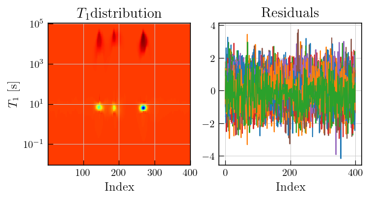
fig,ax = plt.subplots(ncols=2,figsize=(5.5,2.5))
ax[0].pcolor(lspsILT.t[1].flatten(),lspsILT.tau[0].flatten(),lspsILT.g,cmap='jet')
ax[0].set_yscale('log')
ax[0].set_ylabel(r'$T_1$'+' [s]')
ax[0].set_xlabel('Index')
ax[0].set_title(r'$T_1$'+'distribution')


ax[1].plot(lspsILT.residuals.T)
ax[1].set_title('Residuals')
_ = ax[1].set_xlabel('Index')

Without UMFPACK

• This is the default solver if UMFPACK is not installed or is not recognized by scipy.

from scipy.sparse.linalg import spsolve

def no_umfpack_solver(A,b):

    return spsolve(A,b,permc_spec='NATURAL',use_umfpack=False)

lspsILT.invert(solver=no_umfpack_solver)

Starting iterations.
100%, Time elapsed : 1.933 minutes
Done.

Using scikit sparse

• scikit-sparse must be installed : https://pypi.org/project/scikit-sparse/

• Depends on suite-sparse, read more about installation here : https://github.com/scikit-sparse/scikit-sparse

from sksparse.cholmod import cholesky

def skit_solver(A,b):
    factor = cholesky(A)
    x = factor(b)
    return x.flatten()

lspsILT.invert(solver=skit_solver)

Starting iterations.
100%, Time elapsed : 28.529 seconds
Done.

Using Pypardiso

• pypardiso must be installed : https://pypi.org/project/pypardiso/

from pypardiso import spsolve as pardiso_solve

lspsILT.invert(solver=pardiso_solve)

Starting iterations.
100%, Time elapsed : 4.017 minutes
Done.

Using octave

• oct2py must be installed : https://pypi.org/project/oct2py/

• It is possilble to use octave’s solver using oct2Py interface

• However, this approach may show significant performance degradation.

#Use octave's sparse solver using oct2py
from oct2py import Oct2Py

#Create an instance of Oct2Py to interface with Octave
oc = Oct2Py()


def oct_solver(A, b):
    # Create an instance of Oct2Py
    oc = Oct2Py()

    # Send variables A and b to the Octave and solve A\b
    x = oc.feval('mldivide', A, b)

    return x

lspsILT.invert(solver=oct_solver)

Starting iterations.
100%, Time elapsed : 12.683 minutes
Done.