NMR: Weighted Inversion
[1]:
# This file is part of ILTpy examples.
# Author : Dr. Davis Thomas Daniel
# Last updated : 16.02.2026
This example shows steps to do a weighted inversion of NMR data with ILTpy.
It is recommended to familiarize yourself with the first example in the NMR section before continuing.
For more experimental details and discussion about this dataset, please refer to : https://doi.org/10.3390/molecules26216690
Imports
[2]:
# import iltpy
import iltpy as ilt

# other libraries for handling data, plotting
import numpy as np
import matplotlib.pyplot as plt
from scipy.ndimage import uniform_filter
from copy import deepcopy
print(f"ILTpy version: {ilt.__version__}")
ILTpy version: 1.1.0
Data preparation
Load data from text files into numpy arrays
[3]:
# Load pre-processed NMR data.
cpmg_data = np.loadtxt('../../../examples/NMR/weighted_inversion/data.txt')
cpmg_delays = np.loadtxt('../../../examples/NMR/weighted_inversion/delays.txt')

print(f"Data size : {cpmg_data.shape}") # no need for data reduction, since the number of points are less already.
Data size : (128, 350)
Setting noise variance to unity
[4]:
# estimate noise level using the standard deviation of data points in a region with noise.
noise_lvl = np.std(cpmg_data[-1][0:200])
[5]:
# set noise variance to unity
cpmg_data = cpmg_data/noise_lvl
IltPy workflow
Load data
[6]:
# import data into iltpy
ilt_cpmg = ilt.iltload(data=cpmg_data,t=cpmg_delays)
[7]:
ilt_cpmg.data.shape # 128 echo delays and spectra with 350 points.
[7]:
(128, 350)
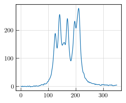
[9]:
# plot to inspect data
fig,ax = plt.subplots(figsize=(5,3.5))
_=ax.plot(ilt_cpmg.data[5]) # spectrum corresponding to 6th echo delay
Initialization and inversion
[10]:
tau = np.logspace(-5,-1,100)
ilt_cpmg.init(tau,kernel=ilt.Exponential())
ilt_cpmg.invert()
Starting iterations ...
100%|██████████| 100/100 [01:48<00:00, 1.09s/it, Convergence=8.28e-03]
Done.
Plot the results
[11]:
chem_shift_axis = np.loadtxt('../../../examples/NMR/weighted_inversion/chem_shift_axis.txt')

fig,ax = plt.subplots(figsize=(7,3.5),ncols=2)
ax[0].pcolor(chem_shift_axis,ilt_cpmg.tau[0].flatten(),ilt_cpmg.g,cmap='jet')
ax[0].set_yscale('log')
ax[0].invert_xaxis()
ax[0].set_xlabel(r'$\delta_{^{1}\mathrm{H}} \mathrm{[ppm]}$')
ax[0].set_ylabel(r'$T_{2} \mathrm{[s]}$')


ax[1].plot(ilt_cpmg.residuals)
ax[1].plot(ilt_cpmg.residuals.mean(axis=1),color='black') # mean of residuals
a1 = ax[1].set_title('Residuals')
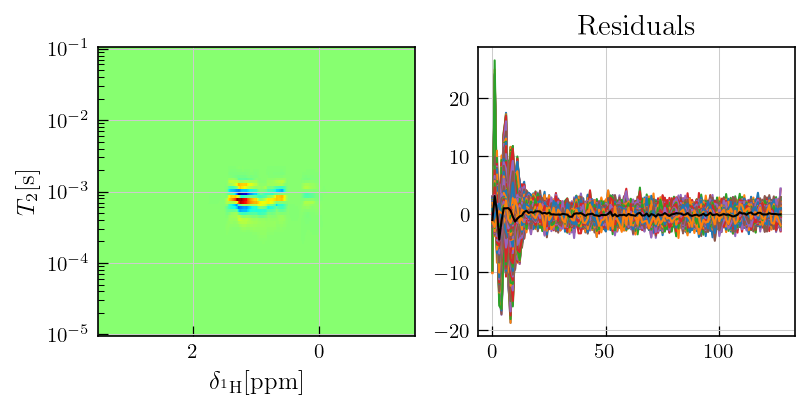
Note
As observed above, the residuals contain sytematic features and deviates from the random noise which is expected in case of a compatible kernel and successful inversion.
Such systematic features may arise from multiple factors such as multiplicative noise or an incompatible kernel.
In case of multiplicative noise, which applies for this particular dataset \(^{1}\), inversion may lead to systematic residuals due to the non-uniform nature of the noise.
Addtionally, oscillatory features in CPMG data may not be fit with an exponential kernel. In a weighted information such features are treated as noise as shown below.
For the weighted inversion, the residuals from an intial inversion are used to estimate a weight matrix for data weighting.
This weight matrix is iteratively updated using the residuals from the previous inversion until the weighted residuals represent random noise, devoid of systematic features.
Merz et al. Molecules, 2021, 26, 6690.
Weighted inversions
[12]:
# Each inversion uses the residuals from the previous inversion:


# first weighted inversion
ilt_cpmg_w = deepcopy(ilt_cpmg) # make a copy of the first IltData object
sigma = np.sqrt(uniform_filter(ilt_cpmg.residuals**2,size=3,mode='constant')) # Estimate the weighting matrix from the residuals, size refers to window size.
ilt_cpmg_w.init(sigma=sigma) # Intialize, rest of the parameters like tau, kernel is retained from the previous IltData object.
ilt_cpmg_w.invert() # invert

# Iteratively update the weighting matrix by using the residuals of the previous inversion and invert (here it is done 2 more times)
ilt_cpmg_w1 = deepcopy(ilt_cpmg)
sigma = np.sqrt(uniform_filter(ilt_cpmg_w.residuals**2,size=3,mode='constant'))
ilt_cpmg_w1.init(sigma=sigma)
ilt_cpmg_w1.invert()

ilt_cpmg_w2 = deepcopy(ilt_cpmg)
sigma = np.sqrt(uniform_filter(ilt_cpmg_w1.residuals**2,size=3,mode='constant'))
ilt_cpmg_w2.init(sigma=sigma)
ilt_cpmg_w2.invert()
Starting iterations ...
100%|██████████| 100/100 [01:54<00:00, 1.15s/it, Convergence=4.72e-03]
Done.
Starting iterations ...
100%|██████████| 100/100 [01:43<00:00, 1.04s/it, Convergence=3.39e-04]
Done.
Starting iterations ...
100%|██████████| 100/100 [01:43<00:00, 1.03s/it, Convergence=6.31e-04]
Done.
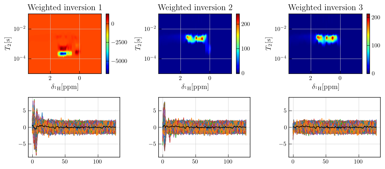
[15]:
# Plot the results
fig,ax = plt.subplots(ncols=3,nrows=2,figsize=(12,5.5))

inv_list = [ilt_cpmg_w,ilt_cpmg_w1,ilt_cpmg_w2]

for i,title in zip(range(3),['Weighted inversion 1','Weighted inversion 2','Weighted inversion 3']):
    g_bc=ax[0,i].pcolor(chem_shift_axis,inv_list[i].tau[0].flatten(),inv_list[i].g,cmap='jet')
    ax[0,i].set_yscale('log')
    ax[0,i].invert_xaxis()
    ax[0,i].set_ylabel(r'$T_{2} \mathrm{[s]}$')
    ax[0,i].set_xlabel(r'$\delta_{^{1}\mathrm{H}} \mathrm{[ppm]}$')
    ax[0,i].set_title(title)
    fig.colorbar(g_bc,ax=ax[0,i])


for i in range(3):
    ax[1,i].plot(inv_list[i].residuals/inv_list[i].sigma)
    ax[1,i].plot((inv_list[i].residuals/inv_list[i].sigma).mean(axis=1),'k')
    ax[1,i].set_ylim((-9,9))

fig.tight_layout()