Bruker EPR data, EPRpy and ILTpy

# This file is part of ILTpy examples.
# Author : Dr. Davis Thomas Daniel
# Last updated : 16.06.2025

• This example shows an ILTpy workflow involving EPR data acuqired on a Bruker spectrometer, reading it using eprpy and then ILT analysis using ILTpy.

• It is recommended to familiarize yourself with the first example in the EPR section before continuing.

• eprpy is a python library for reading EPR data stored in Bruker file formats. For more information see eprpy’s documentation.

• The dataset is a field-resolved inversion recovery dataset, the sample is TEMPO radical. The measurement was done at room temperature.

Imports

import eprpy as epr # eprpy
import iltpy as ilt # iltpy
import numpy as np # numpy
import matplotlib.pyplot as plt # matplotlib

print("eprpy version: ",epr.__version__)
print("ILTpy version: ",ilt.__version__)

eprpy version:  0.9.0a8
ILTpy version:  1.1.0

Read the Bruker data using eprpy

epr_data = epr.load("../../../examples/EPR/bruker_data_IR/T1_VS_FIELD.DSC")

data,t,field_vals = epr_data.data.real,epr_data.x,epr_data.y # extract real data, echo delays, and field values

print(f"Data shape : {data.shape}")
print(f"Number of delays : {t.shape}")
print(f"Number of field values: {field_vals.shape}")

Data shape : (128, 512)
Number of delays : (512,)
Number of field values: (128,)

# note that iltpy requires the dimension which is to be inverted to be the first in case of inversions where both dimensions are not inverted.

Data preparation

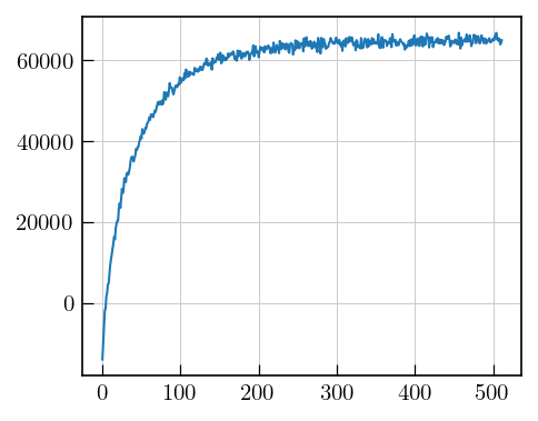
plt.plot(data[64]) # 64th recovery delay

[<matplotlib.lines.Line2D at 0x139335be0>]

# set noise variance to unity by finding a noise region and its standard deviation
noise = np.std(data[0][0:200])

print(f"SD: {noise}")

data = data/noise

SD: 791.9111297992977

# iltpy expects the dimension to be inverted to be the first, so we transpose the data
data = data.T # new shape : (512,128)

ILTpy workflow

Load the data

ilt_data = ilt.iltload(data=data,t=t)

Initialize and invert

ilt_data.init(tau = np.logspace(2,8,100),kernel=ilt.Exponential())

ilt_data.invert()

Starting iterations ...

100%|██████████| 100/100 [00:38<00:00,  2.58it/s, Convergence=1.21e-03]

Done.

Plot the results

import numpy as np
import matplotlib.pyplot as plt
# Prepare the data
x = field_vals/10 # convert Gauss to mT
y = np.log10(ilt_data.tau[0].flatten()/1000) # convert from ns to µs
Z = -ilt_data.g  # Relaxation distribution, we use the negative since this is an inversion recovery dataset

X, Y = np.meshgrid(x, y)
fig = plt.figure(figsize=(8*0.8, 6*0.8))
ax = fig.add_subplot(111, projection='3d')
ax.view_init(elev=50, azim=-35)
surf = ax.plot_surface(X, Y, Z, cmap='jet', edgecolor='none', antialiased=True)
ax.set_xlabel("Magnetic field [mT]",fontsize=10)
ax.set_ylabel(r'$log(T_{1}/ \mu s)$',fontsize=10)
fig.colorbar(surf, ax=ax, shrink=0.5)
plt.tight_layout()
plt.show()

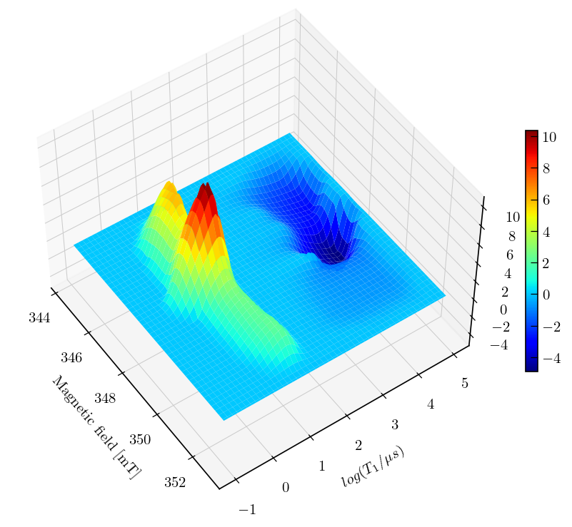
Note

• Inversion recovery curves may exhibit non-zero baselines, which may be interpreted by the algorithm as a slow relaxing component.

• This artefact manifests in the obtained relaxation distribution as a negative peak with a long relaxation time constant, as seen above.

• You can separate this artifact from the real feature by defining a tau vector which has its maximum farther away from the feature of interest.

• The artefact can also be removed by using the static baseline feature as shown below using the sb parameter (available from v.1.1.0)

Static baseline

# we only want the static baseline feature to be applied in the relaxation dimension, not the spectral dimension
# we specify True in the IR dimensions and False for the other.
ilt_data.init(tau = np.logspace(2,8,100),kernel=ilt.Exponential(),parameters={"sb":[True,False]})
ilt_data.invert()

Starting iterations ...

100%|██████████| 100/100 [00:49<00:00,  2.03it/s, Convergence=3.72e-05]

Done.

Note

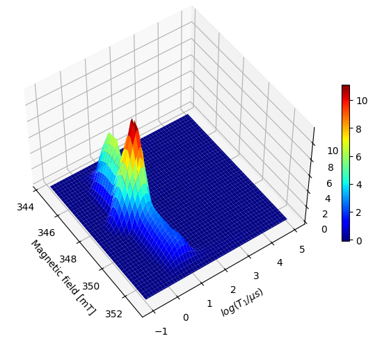
• By specifiying sb=[True, False], we fit the baseline in the inversion recovery dimension using a single point and it no longer appears as an artefact in the resulting distribution.

• Note that the actual features do not change their position.

• It is recommended to review the distribution both with and without the static baseline feature enabled and compare them to ensure the actual features are accurately reproduced in the version where the static baseline is active.

import numpy as np
import matplotlib.pyplot as plt
# Prepare the data
x = field_vals/10 # convert Gauss to mT
y = np.log10(ilt_data.tau[0].flatten()/1000) # convert from ns to µs

# since we use sb as a parameter, an extra point is added to the distribution, we skip this point while plotting since it only fits the baseline.
Z = -ilt_data.g[:-1,:]  # Relaxation distribution, we use the negative since this is an inversion recovery dataset

X, Y = np.meshgrid(x, y)
fig = plt.figure(figsize=(8*0.8, 6*0.8))
ax = fig.add_subplot(111, projection='3d')
ax.view_init(elev=50, azim=-35)
surf = ax.plot_surface(X, Y, Z, cmap='jet', edgecolor='none', antialiased=True)
ax.set_xlabel("Magnetic field [mT]",fontsize=10)
ax.set_ylabel(r'$log(T_{1}/ \mu s)$',fontsize=10)
fig.colorbar(surf, ax=ax, shrink=0.5)
plt.tight_layout()
plt.show()

Note

• By specifiying sb=[True, False], we fit the baseline in the inversion recovery dimension using a single point and it no longer appears as an artefact in the resulting distribution.

• Note that the actual features do not change their position.

• It is recommended to review the distribution both with and without the static baseline feature enabled and compare them to ensure the actual features are accurately reproduced in the version where the static baseline is active.