3D Data - 3D Inversion
[1]:
# This file is part of ILTpy examples.
# Author : Dr. Davis Thomas Daniel
# Last updated : 16.02.2026
This example shows how to do a 3D inversion (all dimensions are inverted) using ILTpy. Please familiarize yourself with 1D and 2D inversions with ILTpy first.
For this example, we will first simulate some synthetic data representing a \(T_{1}\)-\(T_{2}\)-\(D\) (Longitudinal relaxation-Transverse Relaxation-Diffusion) data set and then test if ILTpy reliably reproduces the simulated distribution in the presence of noise.
We will also compare the results with and without data compression.
This example was run on a machine with Apple M1 processor (8 cores) and 16 GB of memory.
Imports
[2]:
import iltpy as ilt
import numpy as np
import matplotlib.pyplot as plt

print(f"ILTpy version: {ilt.__version__}")
ILTpy version: 1.1.0
Generating synthetic data
The true distribution
First, we define a function
gaussian_3dto generate gaussians in 3D space.We define three dimensions for our true distribution, e.g. \(T_{1}\) along dimension 0, \(T_{2}\) along dimension 1 and diffusion constants along dimension 2.
We generate distributions based on these ranges of constants.
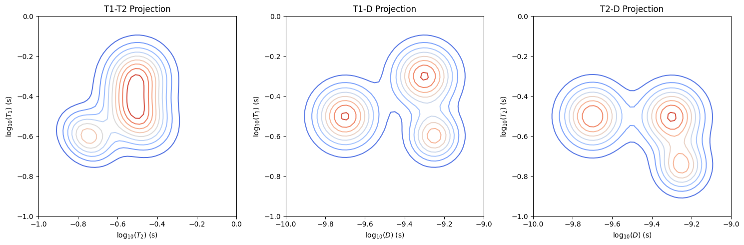
In total, we simulate three components, two of them are not clearly resolved in \(T_{1}\)-\(T_{2}\) dimension but are resolved in the \(T_{1}\)-D and \(T_{2}\)-D dimensions.
[3]:
# Define a function to make 3d gaussians

def gaussian_3d(x, y, z, cx, cy, cz, sx, sy, sz, curve_amp=None, curve_freq=None, curve_axis="y"):
    """
    3D Gaussian with optional sinusoidal deformation along a chosen axis.
    The function evaluates a Gaussian centered at (cx, cy, cz) with standard deviations
    (sx, sy, sz) along the respective axes.
    """
    if curve_amp is not None and curve_freq is not None:
        if curve_axis == "x":
            cx = cx + curve_amp * np.sin(curve_freq * (y - cy))
        elif curve_axis == "y":
            cy = cy + curve_amp * np.sin(curve_freq * (x - cx))
        elif curve_axis == "z":
            cz = cz + curve_amp * np.sin(curve_freq * (x - cx))

    return np.exp(-(((x - cx) ** 2) / (2 * sx ** 2)
                  + ((y - cy) ** 2) / (2 * sy ** 2)
                  + ((z - cz) ** 2) / (2 * sz ** 2)))


# range of T1,T2 and diffusion constants
T1_axis = np.logspace(-1, 0, 50)  # e.g. T1 constants
T2_axis = np.logspace(-1, 0, 50)  # e.g. T2 constants
D_axis = np.logspace(-10, -9, 50)  # e.g. Diffusion constants

# Generate a grid
T1g, T2g, Dg = np.meshgrid(T1_axis, T2_axis, D_axis, indexing='ij')

# Generate the true distribution
dist_3d = (
        gaussian_3d(np.log10(T1g), np.log10(T2g), np.log10(Dg),
                   -0.3, -0.5, -9.3,
                   0.1, 0.1, 0.1)
        +
        gaussian_3d(np.log10(T1g), np.log10(T2g), np.log10(Dg),
                   -0.5, -0.5,-9.7,
                   0.1, 0.1, 0.1,curve_amp=-0.1,curve_freq=2)
        +
        gaussian_3d(np.log10(T1g), np.log10(T2g), np.log10(Dg),
                   -0.6, -0.75,-9.25,
                   0.08, 0.08, 0.08,curve_amp=-0.1,curve_freq=2))
[4]:
print(f"True distribution data shape : {dist_3d.shape}")
True distribution data shape : (50, 50, 50)
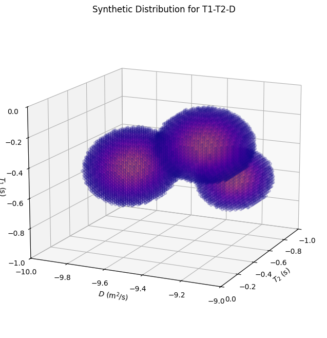
Visualize the true distribution
[5]:
fig = plt.figure(figsize=(8, 8))
ax = fig.add_subplot(111, projection='3d')

threshold = 0.05
mask = (dist_3d > threshold)
scatter = ax.scatter(np.log10(T2g)[mask], np.log10(Dg)[mask], np.log10(T1g)[mask],
                    c=dist_3d[mask], cmap='plasma', s=50, alpha=0.2, marker='.')


ax.set_xlim(-1, 0)   # T2
ax.set_ylim(-10, -9)   # D
ax.set_zlim(-1, 0)  # T1
ax.set_xlabel(r"$T_2$ (s)")
ax.set_ylabel(r"$D$ (m$^2$/s)")
ax.set_zlabel(r"$T_1$ (s)",labelpad=1)
ax.view_init(elev=15, azim=25)

_=ax.set_title('Synthetic Distribution for T1-T2-D', fontsize=12)
Visualize sum projections of true distribution
[6]:
fig, ax = plt.subplots(1, 3, figsize=(15, 5))

# T1 vs T2 projection (sum over D)
data_T1T2 = np.sum(dist_3d, axis=2)
c0 = ax[0].contour(np.log10(T2_axis),np.log10(T1_axis),data_T1T2,cmap='coolwarm',levels=10)
ax[0].set_xlabel(r'log$_{10}(T_2)$ (s)')
ax[0].set_ylabel(r'log$_{10}(T_1)$ (s)')
ax[0].set_title('T1-T2 Projection')

# T1 vs D projection (sum over T2)
data_T1D = np.sum(dist_3d, axis=1)
c1 = ax[1].contour(np.log10(D_axis),np.log10(T1_axis),data_T1D,cmap='coolwarm',levels=10)
ax[1].set_xlabel(r'log$_{10}(D)$ (m$^2$/s)')
ax[1].set_ylabel(r'log$_{10}(T_1)$ (s)')
ax[1].set_title('T1-D Projection')

# T2 vs D projection (sum over T1)
data_T2D = np.sum(dist_3d, axis=0)
c2 = ax[2].contour(np.log10(D_axis),np.log10(T2_axis),data_T2D,cmap='coolwarm',levels=10)
ax[2].set_xlabel(r'log$_{10}(D)$ (m$^2$/s)')
ax[2].set_ylabel(r'log$_{10}(T_2)$ (s)')
ax[2].set_title('T2-D Projection')

plt.tight_layout()
Generate time-domain data
[7]:
# experimental delays, timings etc.
t1_delays = np.logspace(-1, 0, 14).reshape((-1,1))  # s, e.g. inversion recovery delays
t2_delays =  np.logspace(-1, 0, 14).reshape((-1,1))  # s, e.g. cpmg echo delays
b_vals = np.logspace(8.5, 9.8, 14).reshape((-1,1))  # s/m^2, e.g. b_values
[8]:
# Define kernels for each dimension
K_T1 = np.exp(-t1_delays / T1_axis)
K_T2 = np.exp(-t2_delays / T2_axis)
K_D  = np.exp(-b_vals * D_axis)

snr = 100
# Contract kernels with the 3D distribution to generate time-domain data
syn_data_3D = snr*np.einsum('at, tpd, bp, cd -> abc',
                        K_T1, dist_3d, K_T2, K_D)

# Add Gaussian noise to simulate experimental uncertainty in real NMR acquisitions
# This produces a synthetic dataset with a noise variance of unity.
np.random.seed(2505)
syn_data_3D += np.random.randn(*syn_data_3D.shape)
print("Time-domain data shape:", syn_data_3D.shape)
Time-domain data shape: (14, 14, 14)
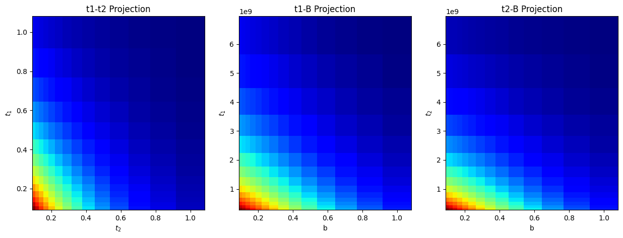
Visualize time-domain data
[9]:
fig, ax = plt.subplots(1, 3, figsize=(15, 5))

# T1 vs T2 projection (sum over D)
data_T1T2 = np.sum(syn_data_3D, axis=2)
ax[0].pcolor(t2_delays.flatten(),t1_delays.flatten(),data_T1T2,cmap='jet')
ax[0].set_xlabel(r'$t_{2}$')
ax[0].set_ylabel(r'$t_{1}$')
ax[0].set_title('t1-t2 Projection')

# T1 vs D projection (sum over T2)
data_T1D = np.sum(syn_data_3D, axis=1)
ax[1].pcolor(t1_delays.flatten(),b_vals.flatten(),data_T1D,cmap='jet')
ax[1].set_xlabel("b")
ax[1].set_ylabel(r'$t_{1}$')
ax[1].set_title('t1-B Projection')

# T2 vs D projection (sum over T1)
data_T2D = np.sum(syn_data_3D, axis=0)
ax[2].pcolor(t2_delays.flatten(),b_vals.flatten(),data_T2D,cmap='jet')
ax[2].set_xlabel("b")
ax[2].set_ylabel(r'$t_{2}$')
ax[2].set_title('t2-B Projection')
[9]:
Text(0.5, 1.0, 't2-B Projection')
[10]:
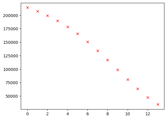
# individual traces can be visualized too.
_=plt.plot(syn_data_3D[0,0,:],'xr') # diffusion decay corresponding to first t1 delay, first t2 delay
Iltpy Workflow
Load data
[11]:
# load data into an IltData object by specifying the data and the input sampling arrays
# In the first, second and third dimension, we use the simulated delays, b value as input sampling arrays
ilt_3d = ilt.iltload(data=syn_data_3D,t=[t1_delays,t2_delays,b_vals])
Initialize
[12]:
tau1,tau2,tau3 =  np.logspace(-1, 0, 26),np.logspace(-1, 0, 26),np.logspace(-10, -9, 26) # define output sampling for ILT
parameters={"alt_g":6,"maxloop":50} # Here with alt_g = 6, we use a different variation of the algorithm, whcih is faster in cases where all dimensions are inverted.
ilt_3d.init(tau=[tau1,tau2,tau3],kernel=[ilt.Exponential(),ilt.Exponential(),ilt.Diffusion()],verbose=2,parameters=parameters) # we use in-built kernels from ILTpy.
Initializing...
Reading fit parameters...
Setting fit parameters...
Initializing fit parameters...
Initializing kernel matrices...
    Initializing kernel matrix in dimension 0...
    Initializing kernel matrix in dimension 1...
    Initializing kernel matrix in dimension 2...
    Kernel initialization done.
Initializing regularization matrices...
   Calculating constant, regularization matrices...
   Calculating diagonal matrices...
   Calculating amplitude regularization...
   Regularization matrices initialization done.
Initialization took 0.225 seconds.
Invert
[13]:
ilt_3d.invert()
Starting iterations ...
100%|██████████| 50/50 [19:40<00:00, 23.61s/it, Convergence=5.14e-04]
Done.
[ ]:
Plot convergence
[14]:
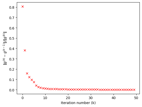
# we can check if the convergence was achieved within 50 iterations by plotting the convergence history
plt.plot(ilt_3d.convergence,'xr')
plt.xlabel("Iteration number (k)")
_=plt.ylabel(r'$\| g^{(k)} - g^{(k-1)} \| / \| g^{(k)} \|$')
Plot results and compare
[15]:
# in this plot we compare the true and ILT-derived distributions.

fig, ax = plt.subplots(2, 3, figsize=(15, 10))

# ILT distribution plots (Top row)

# T1 vs T2 projection (sum over D)
data_T1T2 = np.sum(ilt_3d.g, axis=2)
c0 = ax[0, 0].contourf(np.log10(tau2),np.log10(tau1),data_T1T2,cmap='jet',levels=10)
ax[0, 0].set_xlabel(r'log$_{10}(T_2)$ (s)')
ax[0, 0].set_ylabel(r'log$_{10}(T_1)$ (s)')
ax[0, 0].set_title('ILTpy: T1-T2 Projection')

# T1 vs D projection (sum over T2)
data_T1D = np.sum(ilt_3d.g, axis=1)
c1 = ax[0, 1].contourf(np.log10(tau3),np.log10(tau1),data_T1D,cmap='jet',levels=10)
ax[0, 1].set_xlabel(r'log$_{10}(D)$ (m$^2$/s)')
ax[0, 1].set_ylabel(r'log$_{10}(T_1)$ (s)')
ax[0, 1].set_title('ILTpy: T1-D Projection')

# T2 vs D projection (sum over T1)
data_T2D = np.sum(ilt_3d.g, axis=0)
c2 = ax[0, 2].contourf(np.log10(tau3),np.log10(tau2),data_T2D,cmap='jet',levels=10)
ax[0, 2].set_xlabel(r'log$_{10}(D)$ (m$^2$/s)')
ax[0, 2].set_ylabel(r'log$_{10}(T_2)$ (s)')
ax[0, 2].set_title('ILTpy: T2-D Projection')

# True distribution plots (Bottom row)

# T1 vs T2 projection (sum over D)
data_T1T2_true = np.sum(dist_3d, axis=2)
c3 = ax[1, 0].contourf(np.log10(T2_axis), np.log10(T1_axis), data_T1T2_true, cmap='coolwarm', levels=10)
ax[1, 0].set_xlabel(r'log$_{10}(T_2)$ (s)')
ax[1, 0].set_ylabel(r'log$_{10}(T_1)$ (s)')
ax[1, 0].set_title('True: T1-T2 Projection')

# T1 vs D projection (sum over T2)
data_T1D_true = np.sum(dist_3d, axis=1)
c4 = ax[1, 1].contourf(np.log10(D_axis), np.log10(T1_axis), data_T1D_true, cmap='coolwarm',levels=10)
ax[1, 1].set_xlabel(r'log$_{10}(D)$ (m$^2$/s)')
ax[1, 1].set_ylabel(r'log$_{10}(T_1)$ (s)')
ax[1, 1].set_title('True: T1-D Projection')

# T2 vs D projection (sum over T1)
data_T2D_true = np.sum(dist_3d, axis=0)
c5 = ax[1, 2].contourf(np.log10(D_axis), np.log10(T2_axis), data_T2D_true, cmap='coolwarm', levels=10)
ax[1, 2].set_xlabel(r'log$_{10}(D)$ (m$^2$/s)')
ax[1, 2].set_ylabel(r'log$_{10}(T_2)$ (s)')
ax[1, 2].set_title('True: T2-D Projection')

plt.tight_layout()
plt.show()
[16]:
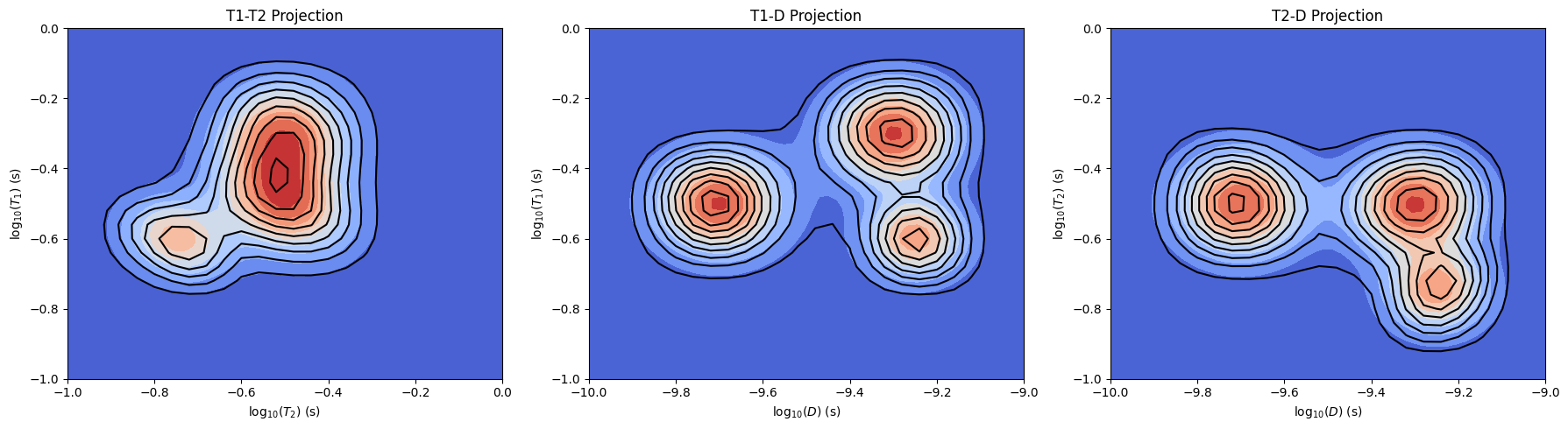
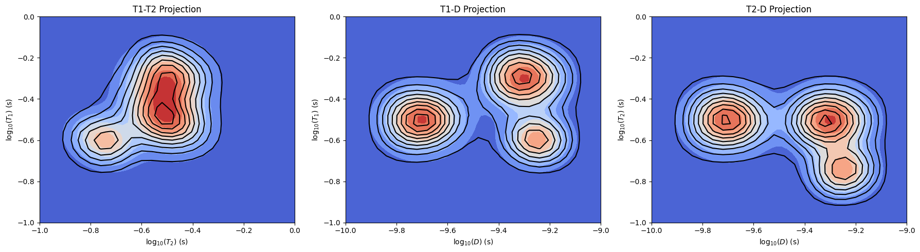
# We can overlay the predicted distributions on top of the true distributions,
# In this plot, filled contours are the true distributions,
# with unfilled black contours representing the distributions obtained from ILTpy overlaid on top

fig, ax = plt.subplots(1, 3, figsize=(18, 5))

# T1 vs T2 Projection
data_T1T2_true = np.sum(dist_3d, axis=2)
data_T1T2_ilt = np.sum(ilt_3d.g, axis=2)

cf0 = ax[0].contourf(np.log10(T2_axis), np.log10(T1_axis), data_T1T2_true, cmap='coolwarm', levels=10)
c0 = ax[0].contour(np.log10(tau2), np.log10(tau1), data_T1T2_ilt, colors='black', levels=10)

ax[0].set_xlabel(r'log$_{10}(T_2)$ (s)')
ax[0].set_ylabel(r'log$_{10}(T_1)$ (s)')
ax[0].set_title('T1-T2 Projection')

# T1 vs D Projection
data_T1D_true = np.sum(dist_3d, axis=1)
data_T1D_ilt = np.sum(ilt_3d.g, axis=1)

cf1 = ax[1].contourf(np.log10(D_axis), np.log10(T1_axis), data_T1D_true, cmap='coolwarm', levels=10)
c1 = ax[1].contour(np.log10(tau3), np.log10(tau1), data_T1D_ilt, colors='black', levels=10)

ax[1].set_xlabel(r'log$_{10}(D)$ (m$^2$/s)')
ax[1].set_ylabel(r'log$_{10}(T_1)$ (s)')
ax[1].set_title('T1-D Projection')


# T2 vs D Projection
data_T2D_true = np.sum(dist_3d, axis=0)
data_T2D_ilt = np.sum(ilt_3d.g, axis=0)

cf2 = ax[2].contourf(np.log10(D_axis), np.log10(T2_axis), data_T2D_true, cmap='coolwarm', levels=10)
c2 = ax[2].contour(np.log10(tau3), np.log10(tau2), data_T2D_ilt, colors='black', levels=10)

ax[2].set_xlabel(r'log$_{10}(D)$ (m$^2$/s)')
ax[2].set_ylabel(r'log$_{10}(T_2)$ (s)')
ax[2].set_title('T2-D Projection')


plt.tight_layout()
plt.show()
From the plots above, we see that all the components in simulated distributions are extracted at the correct positions (T1,T2 and D constants) after the inversion. Due to noise and smaller number of points in the output sampling, the distributions from ILT are broader than the simulated distributions.
Appendix : With data compression
Now, we repeat the inversion with data compression using singular value decomposition.
[17]:
from copy import deepcopy
[18]:
ilt_3dc = deepcopy(ilt_3d) # make a copy of the previous iltdata
Initialize
We employ compression in all three dimensions, with 7 singular values using the parameters
compressands
[19]:
tau1,tau2,tau3 =  np.logspace(-1, 0, 26),np.logspace(-1, 0, 26),np.logspace(-10, -9, 26) # define output sampling for ILT, same as before

# Here with alt_g = 6, we use a different variation of the algorithm, which is faster when all dimensions are inverted.
# We employ compression in all three dimensions, with 7 singular values
parameters={"alt_g":6,"maxloop":50,"compress":[True,True,True],"s":[4,4,4]}
# we use in-built kernels from ILTpy.
ilt_3dc.init(tau=[tau1,tau2,tau3],kernel=[ilt.Exponential(),ilt.Exponential(),ilt.Diffusion()],verbose=2,parameters=parameters)
Initializing...
Reading fit parameters...
Setting fit parameters...
Initializing fit parameters...
Initializing kernel matrices...
    Initializing kernel matrix in dimension 0...
    Initializing kernel matrix in dimension 1...
    Initializing kernel matrix in dimension 2...
    Kernel initialization done.
Initializing regularization matrices...
   Calculating constant, regularization matrices...
   Calculating diagonal matrices...
   Calculating amplitude regularization...
   Regularization matrices initialization done.
Initialization took 0.032 seconds.
Invert
[20]:
ilt_3dc.invert()
Starting iterations ...
100%|██████████| 50/50 [12:29<00:00, 15.00s/it, Convergence=1.29e-03]
Done.
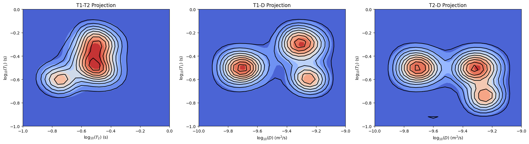
We can overlay the predicted distributions on top of the true distribution to compare.
In this plot, filled contours are the true distribution, with unfilled black countours representing the distributions obtained from ILTpy with data compression overlaid on top
Plot results
[21]:
fig, ax = plt.subplots(1, 3, figsize=(18, 5))

# T1 vs T2 Projection
data_T1T2_true = np.sum(dist_3d, axis=2)
data_T1T2_ilt = np.sum(ilt_3dc.g, axis=2)

cf0 = ax[0].contourf(np.log10(T2_axis), np.log10(T1_axis), data_T1T2_true, cmap='coolwarm', levels=10)
c0 = ax[0].contour(np.log10(tau2), np.log10(tau1), data_T1T2_ilt, colors='black', levels=10)

ax[0].set_xlabel(r'log$_{10}(T_2)$ (s)')
ax[0].set_ylabel(r'log$_{10}(T_1)$ (s)')
ax[0].set_title('T1-T2 Projection')

# T1 vs D Projection
data_T1D_true = np.sum(dist_3d, axis=1)
data_T1D_ilt = np.sum(ilt_3dc.g, axis=1)

cf1 = ax[1].contourf(np.log10(D_axis), np.log10(T1_axis), data_T1D_true, cmap='coolwarm', levels=10)
c1 = ax[1].contour(np.log10(tau3), np.log10(tau1), data_T1D_ilt, colors='black', levels=10)

ax[1].set_xlabel(r'log$_{10}(D)$ (m$^2$/s)')
ax[1].set_ylabel(r'log$_{10}(T_1)$ (s)')
ax[1].set_title('T1-D Projection')


# T2 vs D Projection
data_T2D_true = np.sum(dist_3d, axis=0)
data_T2D_ilt = np.sum(ilt_3dc.g, axis=0)

cf2 = ax[2].contourf(np.log10(D_axis), np.log10(T2_axis), data_T2D_true, cmap='coolwarm', levels=10)
c2 = ax[2].contour(np.log10(tau3), np.log10(tau2), data_T2D_ilt, colors='black', levels=10)

ax[2].set_xlabel(r'log$_{10}(D)$ (m$^2$/s)')
ax[2].set_ylabel(r'log$_{10}(T_2)$ (s)')
ax[2].set_title('T2-D Projection')

plt.tight_layout()
plt.show()