1D Data - 1D Inversion

# This file is part of ILTpy examples.
# Author : Dr. Davis Thomas Daniel
# Last updated : 25.08.2025

• This example shows how to do a 1D inversion using ILTPy.

• For this example, we will first simulate some synthetic data using Kohlrausch–Williams–Watts function with some postive and negative peaks.

• This example was run on a machine with Apple M1 processor (8 core CPU) and 16 GB of memory.

Imports

import iltpy as ilt
import numpy as np
import matplotlib.pyplot as plt

print(f"ILTpy version: {ilt.__version__}")

ILTpy version: 1.0.0

Generating synthetic data

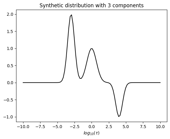
The true distribution

def gaussian(x, mu, sigma, amplitude):
   return amplitude * np.exp(-0.5 * ((x - mu) / sigma) ** 2)

# Generate synthetic spectrum
tau = np.linspace(-10, 10, 100)
components = [-3, 0, 4]
sigmas = [0.5, 0.7, 0.5]
amplitudes = [2,1,-1]

dist1d = np.zeros_like(tau)

# Add multiple Gaussian components to the spectrum
for mu, sigma, amplitude in zip(components, sigmas, amplitudes):
   dist1d += gaussian(tau, mu, sigma, amplitude)

Visualize the true distribution

# Plot the result
plt.plot(tau, dist1d,'k')
plt.title('Synthetic distribution with 3 components')
plt.xlabel(r'$log_{10}(\tau)$')
plt.show()

Generate time-domain data

## Time domain data :
#timing
t_syn = np.logspace(-10,10,1024).reshape((-1,1))
# kernel matrix
K_matrix = ilt.Exponential().kernel(t_syn,10**tau)
snr = 2
syn_data_1D = snr * K_matrix @ dist1d

## add noise
np.random.seed(2505)
syn_data_1D += np.random.randn(len(t_syn))

Iltpy Workflow

Load data

# Load the data into iltpy using iltload
ilt_1d = ilt.iltload(data=syn_data_1D, t=t_syn)

Initialize

# Specify parameters and  initialize inversion
tau = np.logspace(-10, 10, 100) # output sampling points
ilt_1d.init(tau=tau, kernel=ilt.Exponential())

Invert

ilt_1d.invert()

Starting iterations ...

100%|██████████| 100/100 [00:00<00:00, 874.39it/s]

Done.

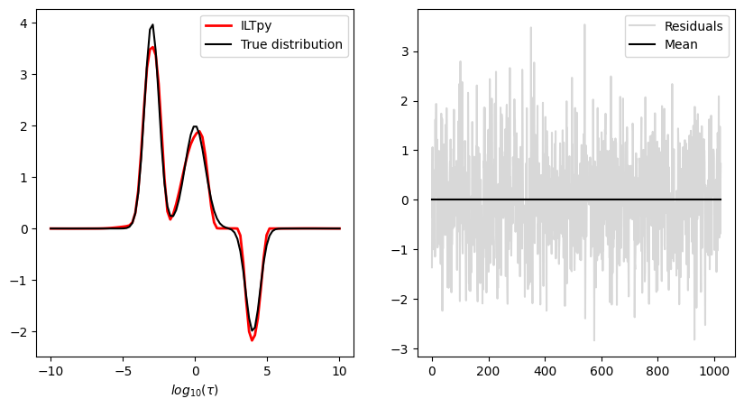
Plot results

fig,ax = plt.subplots(ncols=2,figsize=[10,5])
ax[0].plot(np.log10(tau),ilt_1d.g,label='ILTpy',color='red',linewidth=2)
ax[0].plot(np.log10(tau),dist1d*snr,label='True distribution',color='black')
ax[0].set_xlabel(r'$log_{10}(\tau)$')
ax[0].legend()
ax[1].plot(ilt_1d.residuals,label='Residuals',alpha=0.3,color='grey')
ax[1].plot([ilt_1d.residuals.mean()]*1024,label='Mean',color='black')


ax[1].legend()

<matplotlib.legend.Legend at 0x1184b5590>

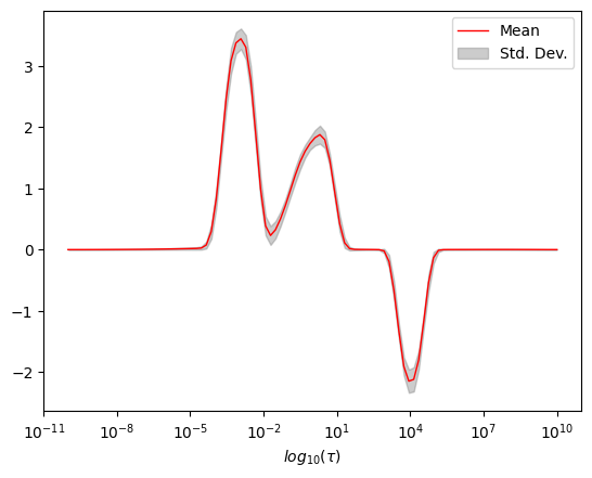
Appendix : Uncertainity Estimation

• iltstats can be used to estimate uncertainty by refitting the initial fit of the data with randomly generated noise vectors and inverting n times.

• To use iltstats, data must be inverted at least once.

• n controls the number of data samples which will be generated and n_jobs controls the number of parallel jobs to create.

ilt_1d.iltstats(n=200,n_jobs=-1) # n_jobs = -1 uses all available processors.

[Parallel(n_jobs=-1)]: Using backend LokyBackend with 8 concurrent workers.
[Parallel(n_jobs=-1)]: Done  34 tasks      | elapsed:    1.7s
[Parallel(n_jobs=-1)]: Done 184 tasks      | elapsed:    5.5s
[Parallel(n_jobs=-1)]: Done 200 out of 200 | elapsed:    5.9s finished

Plot results

fig,ax = plt.subplots()
ax.semilogx(ilt_1d.tau[0].flatten(),ilt_1d.statistics['g_mean'],color='r',linewidth=1,label='Mean')
ax.fill_between(ilt_1d.tau[0].flatten(),*[i for i in ilt_1d.statistics['g_conf_interval']],color='grey',alpha=0.4,label='Std. Dev.')
ax.legend()
_=ax.set_xlabel(r'$log_{10}(\tau)$')

#plt.xlim(1e4,2e6)
#_=plt.ylim(-1,22)