2D Data - Pseudo 2D Inversion
[1]:
# This file is part of IltPy examples.
# Author : Dr. Davis Thomas Daniel
# Last updated : 16.02.2026
This example shows how to do a Pseudo 2D inversion (2D data with first dimension inverted) using IltPy.
For this example, we will first simulate some synthetic data representing a \(T_{2}\) data set.
The first dimension will be the \(T_{2}\) dimension and the second dimension would be e.g the NMR spectrum.
This example was run on a machine with Apple M1 processor (8 cores) and 16 GB of memory.
Imports
[2]:
import iltpy as ilt
import numpy as np
import matplotlib.pyplot as plt
from iltpy.output.plotting import iltplot
from scipy.stats import multivariate_normal

print(f"ILTpy version: {ilt.__version__}")
ILTpy version: 1.1.0
Generating synthetic data
The True distribution
[3]:
## Generate Gaussian distributions
t_constants = [0,0,-1,2,2.2,4.5,3] # relaxation constants (e.g in s)
chemical_shift = [0.8,0,8,2,2.5,5,5] # nmr peaks/resonances (ppm)

# specify peak shapes by adjusting covariances
covariances = [
    [[0.07, 0], [0, 0.01]],
    [[0.07, 0], [0, 0.01]],
    [[0.1, 0], [0, 0.01]],
    [[0.01, 0], [0, 0.1]],
    [[0.1, 0], [0, 0.1]],
    [[0.01, 0], [0, 0.1]],
    [[0.01, 0], [0, 0.1]],
]

# amplitude of resonances
amplitudes = [1,1,1,0.5,1,0.5,0.5]

chemical_shift_axis = np.linspace(-3, 10, 256)
t_delays = np.linspace(-3, 6, 200)

X, Y = np.meshgrid(chemical_shift_axis, t_delays)
pos = np.dstack((X, Y))

dist2d = np.zeros_like(X)
for mean, cov, amp in zip(zip(chemical_shift, t_constants), covariances, amplitudes):
    rv = multivariate_normal(mean, cov)
    dist2d += amp * rv.pdf(pos)

print(f"True distribution data shape : {dist2d.shape}")
True distribution data shape : (200, 256)
Visualize the true distribution
[4]:
plt.figure(figsize=(10, 8))
plt.contourf(X, Y, dist2d, cmap='coolwarm',levels=25)
plt.colorbar()
plt.xlabel('Chemical shift [ppm]')
plt.ylabel('log(T2)')
plt.title('Simulated NMR relaxation distribution')
[4]:
Text(0.5, 1.0, 'Simulated NMR relaxation distribution')
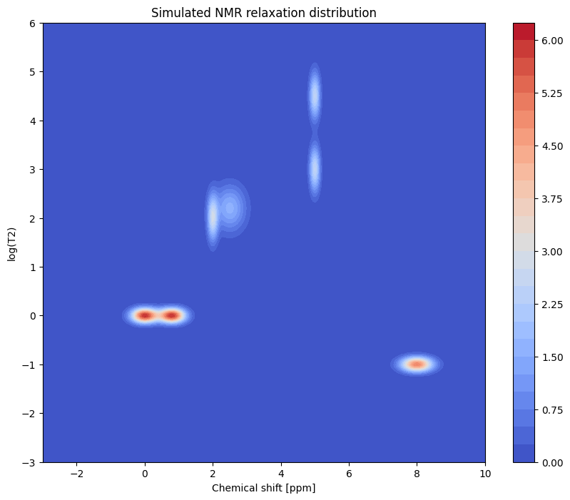
A total of 7 resonance peaks are generated.
Peak close to 0 ppm represents a doublet with the same relaxation time.
Peak at 2 ppm represents the overlap of a broad and narrow peaks with different relaxation behaviour.
Peak at 5 ppm shows two peaks overlapping such that they are not resolved in the spectral dimension but are resolved in the relaxation dimension.
Peak at 8 ppm is a broad single peak, which relaxes the fastest.
Generate time-domain data
[5]:
## Time domain data :
#timing
spectrum_axis = np.linspace(-3, 10, 256).reshape((-1,1)) # same as chemical shift axis
t_syn = np.logspace(-2,7,32).reshape((-1,1)) # experimental timing, such as vclist or vdlist

# kernel matrix
K_matrix1 = ilt.Identity().kernel(spectrum_axis,10**chemical_shift_axis)
K_matrix2 = ilt.Exponential().kernel(t_syn,10**t_delays)

snr = 500
syn_data_2D = snr * K_matrix2 @ dist2d @ K_matrix1.T

## add noise
np.random.seed(2505)
syn_data_2D += np.random.randn(len(t_syn),len(spectrum_axis))
[6]:
syn_data_2D.shape # 32 points in the relaxation dimension and 512 points in the spectrum
[6]:
(32, 256)
Visualize time-domain data
[7]:
plt.plot(chemical_shift_axis,syn_data_2D[0]) # spectrum corresponding to first delay
plt.plot(chemical_shift_axis,syn_data_2D[16]) # spectrum corresponding to intermediate delay
plt.plot(chemical_shift_axis,syn_data_2D[-1]) # spectrum corresponding to last delay
plt.xlabel("Chemical shift [ppm]")

plt.legend(["First delay","Intermediate delay","Last delay"])
[7]:
<matplotlib.legend.Legend at 0x12c1897f0>

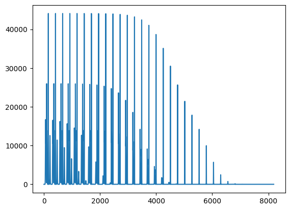
[8]:
_=plt.plot(syn_data_2D.flatten()) # whole dataset flattened
Iltpy Workflow
Load data
[9]:
# load data into an IltData object by specifying the data and the input sampling array (t_syn in this case)
ilt_2d = ilt.iltload(data=syn_data_2D,t=t_syn)
We don’t need to specify the chemical shift axis as input sampling in the second dimension, as we don’t intend to invert the second dimension (see initialization step below).
In this case, ILTpy chooses an array of unit spacing for the second dimension, we can change that by using the
dim_ndimparameter.
Initialize
[10]:
# We can initialize by matching the spacing of the original data, specified by the dim_ndim parameter
# spacing of original chemical shift axis
np.mean(np.diff(chemical_shift_axis))
[10]:
np.float64(0.050980392156862744)
[11]:
ilt_2d.init(tau=np.logspace(-3, 6, 80),kernel=ilt.Exponential(),dim_ndim=np.arange(1,257)/20)
[12]:
print("Input sampling characteristics in second dimension : ")
print(f"Minimum value : {np.min(ilt_2d.t[1])}, Maximum value : {np.max(ilt_2d.t[1])}, Spacing : {np.mean(np.diff(ilt_2d.t[1]))}")
Input sampling characteristics in second dimension :
Minimum value : 0.05, Maximum value : 12.8, Spacing : 0.05
Invert
[13]:
ilt_2d.invert()
Starting iterations ...
100%|██████████| 100/100 [01:01<00:00, 1.62it/s, Convergence=5.66e-04]
Done.
[14]:
iltplot(ilt_2d,transpose_residuals=True)
[14]:
(<Figure size 637x757 with 4 Axes>,
 [<Axes: xlabel='t'>,
  <Axes: ylabel='log($\\tau$)'>,
  <Axes: title={'center': '$r = \\mathbf{Kg}-\\mathbf{s}$'}>])

From the plots above, we see that all the components in simulated distributions are extracted at the correct positions and shapes.
The residuals are random with zero mean, indicating a comptaible kernel and successful inversion.