3D Data - Pseudo 3D Inversion
[1]:
# This file is part of ILTpy examples.
# Author : Dr. Davis Thomas Daniel
# Last updated : 22.08.2025
This example shows how to do a pseudo 3D inversion (3D data with where two dimensions are inverted) using ILTpy. Please familiarize yourself with 1D and 2D inversions with ILTpy first.
For this example, we will first simulate some synthetic data and then see if ILTpy reliably reproduces the simulated distribution in the presence of noise.
We will also compare the results with and without data compression.
This example was run on a machine with Apple M1 processor (8 cores) and 16 GB of memory.
Imports
[2]:
# import iltpy
import iltpy as ilt

# importing libraries for data genration, plotting etc.
import numpy as np
import matplotlib.pyplot as plt
from scipy.stats import multivariate_normal

print(f"ILTpy version: {ilt.__version__}")
ILTpy version: 1.1.0
Generating synthetic data
The true distribution
[3]:
# Initialize an empty array to store synthetic 2D correlation maps
# For instance, the data could have the dimensions: 100 (T1 points) x 100 (T2 points) x 10 (temperatures)

data_3d = np.empty((100,100,10))

# Loop over the last dimension
for j in range(data_3d.shape[2]):

    # We simulate three different components with varying t1,t2 constants, amplitudes, shapes etc.

    # Simulate shift in relaxation times (T1, T2): We shift one pair of components along the T2 axis and another pair of peaks along the T1 axis.
    shift = j/5
    t2_constants = [-0.5, -0.5+shift, 1.5-shift, 1.5]
    shift = j/10
    t1_constants = [0.4+shift, 0, 0, 0.4+shift]

    # Define peak shapes using covariance matrices (controls elongation and orientation of 2D Gaussians)
    covariances = [[[0.05, 0], [0, 0.1]], [[0.01, 0], [0, 0.1]],[[0.01, 0], [0, 0.1]], [[0.05, 0], [0, 0.1]]]

    # Two postive components and one negative
    amplitudes = [-1, -0.5,0.5,1]

    # Define smapling arrays in first and second dimensions
    dim1 = np.linspace(-1.5, 2.5, 100)
    dim2 = np.linspace(-1.5, 2.5, 100)

    X, Y = np.meshgrid(dim1, dim2)
    pos = np.dstack((X, Y))

    # Generate each peak (component) in the T1-T2 space and sum to create the full correlation map
    Z = np.zeros_like(X)
    for mean, cov, amp in zip(zip(t2_constants, t1_constants), covariances, amplitudes):
        rv = multivariate_normal(mean, cov)
        Z += amp * rv.pdf(pos)

    data_3d[:,:,j] = Z
[4]:
print(f"Data size : {data_3d.shape}")
Data size : (100, 100, 10)
Visualize the distributions
[5]:
fig, axes = plt.subplots(2, 5, figsize=(15, 6), constrained_layout=True)

axes = axes.flatten()

for idx in range(10):
    ax = axes[idx]
    im = ax.pcolor(dim1,dim2,data_3d[:, :, idx],
                   cmap='jet')
    ax.set_title(f"Index {idx+1} / 10")
    ax.set_xlabel(r"$T_2$")
    ax.set_ylabel(r"$T_1$")

    plt.colorbar(im, ax=ax, shrink=0.8)

fig.suptitle("Simulated Distributions", fontsize=16)
plt.show()
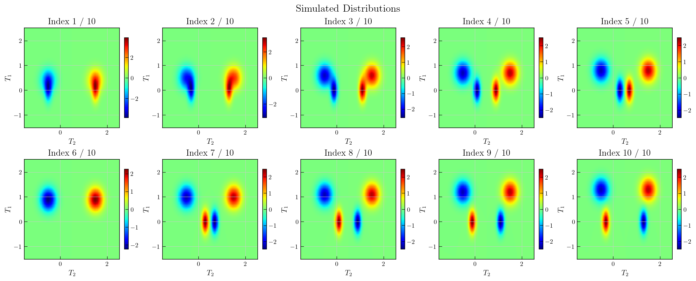
We have generated 4 components (two positive and two negative components) which are intially merged.
Two of the components move along the the \(T_{1}\) axis and and the other two move along \(T_{2}\).
The components moving along \(T_{2}\) merge at index 6, leading to their disappearance as they have opposite signs. The components reappear as they shift again.
Finally, we have four components which are completely resolved at index 10.
Simulation of time-Domain data
[6]:
# Define time axes (e.g., inversion recovery or echo times)
# Timings in T1 or T2 experiments spanning milliseconds to seconds (input sampling)
t_syn1 = np.logspace(-1, 3, 32).reshape((-1, 1))  # T1 recovery delays (e.g., 0.1 s to 1000 s)
t_syn2 = np.logspace(-1, 3, 32).reshape((-1, 1))  # T2 echo delays (e.g., 0.1 ms to 1000 ms)

# Construct exponential decay kernels for inverse Laplace transform (ILT)
# These map relaxation distributions (in log(T1), log(T2)) to time-domain signals
K_matrix1 = np.exp(-t_syn1*1/10**dim1)  # Kernel for T1 axis
K_matrix2 = np.exp(-t_syn2*1/10**dim2)  # Kernel for T2 axis

# Simulate time-domain signal data from 2D relaxation maps
snr = 10  # Signal-to-noise ratio
syn_data_3D = snr * np.einsum('ti,ijz,sj->tsz', K_matrix1, data_3d, K_matrix2)
# Add Gaussian noise to simulate experimental uncertainty in real NMR acquisitions
# This produces a synthetic dataset with a noise variance of unity.
syn_data_3D += np.random.randn(len(t_syn1), len(t_syn2), len(np.linspace(-5, 5, 10)))

print(f"Time-domain data shape : {syn_data_3D.shape}")
Time-domain data shape : (32, 32, 10)
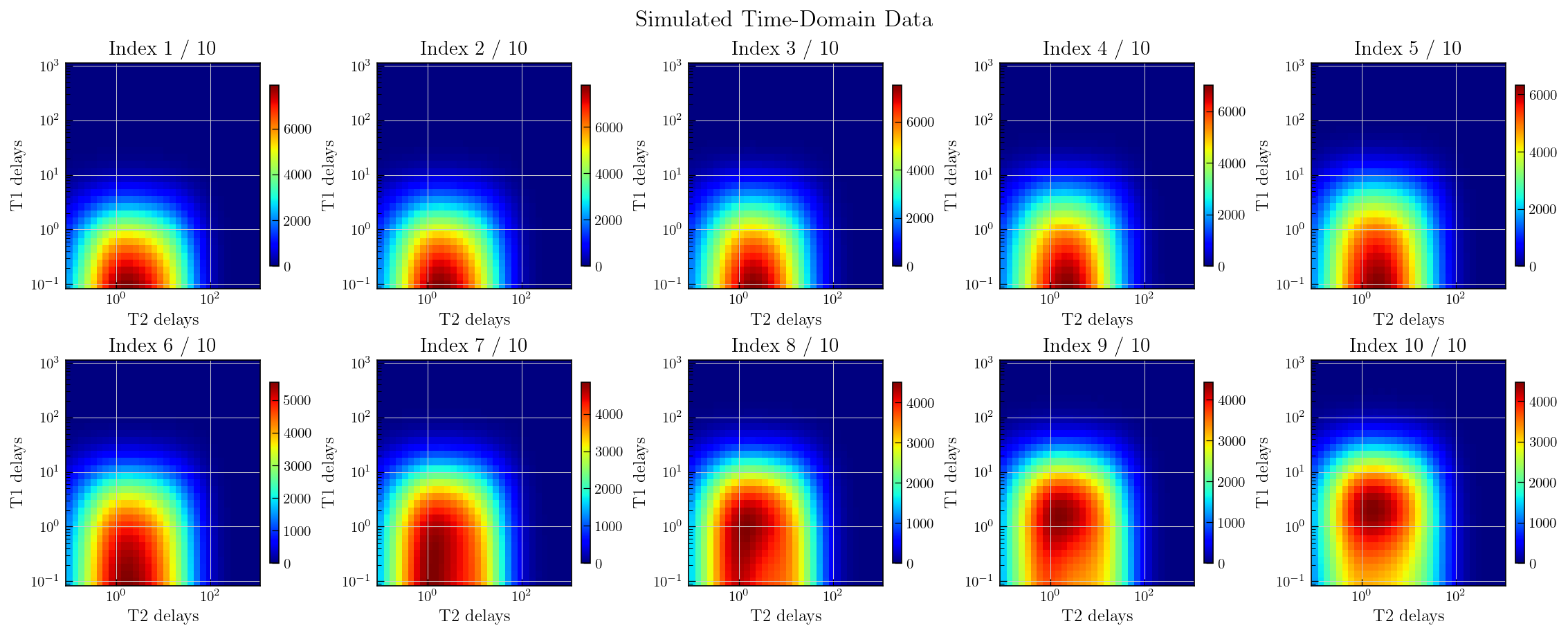
We have generated data with:
32 points in the first dimension: For instance, this could correspond to T1 recovery delays (e.g., inversion recovery or saturation recovery delays), simulated using a logarithmic spacing from 0.1 ms to 1000 ms.
32 points in the second dimension : For instance, this could correspond to T2 echo delays (e.g., echo times), also logarithmically spaced from 0.1 s to 1000 s.
10 points in the third dimension: Represents the variable in the third dimension, e.g. different temperatures.
Visualize the synthetic data
[7]:
fig, axes = plt.subplots(2, 5, figsize=(15, 6), constrained_layout=True)

axes = axes.flatten()

for idx in range(10):
    ax = axes[idx]
    im = ax.pcolor(t_syn1.flatten(),t_syn2.flatten(),syn_data_3D[:, :, idx],
                   cmap='jet')
    ax.set_title(f"Index {idx+1} / 10")
    ax.set_xlabel("T2 delays")
    ax.set_ylabel("T1 delays")
    ax.set_yscale('log')
    ax.set_xscale('log')


    plt.colorbar(im, ax=ax, shrink=0.8)

fig.suptitle("Simulated Time-Domain Data", fontsize=16)
plt.show()
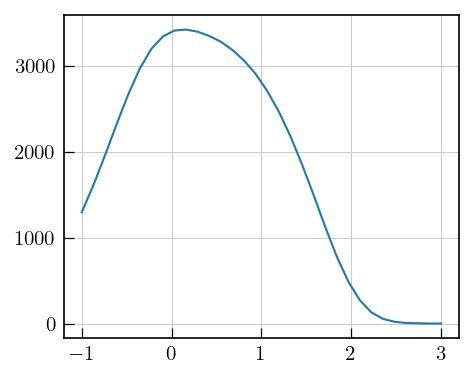
[8]:
# we can also look at individual traces

fig,ax = plt.subplots()

ax.plot(np.log10(t_syn2),syn_data_3D[2,:,-1])
[8]:
[<matplotlib.lines.Line2D at 0x14386ef90>]
ILTpy workflow
Load data
[9]:
# load data into an IltData object by specifying the data and the input sampling arrays
# In the first and second dimension, we use the simulated delays as input sampling arrays
# in the third dimension we use a linearly spaced array
ilt_3d = ilt.iltload(data=syn_data_3D,t=[t_syn1,t_syn2,np.linspace(-25,25,10)])
Initialize
[10]:
# we only invert the first and second dimensions (for instance, T1 and T2 dimensions), but regularize all three.

tau = [np.logspace(-1.5,2.5,40),np.logspace(-1.5,2.5,40),np.linspace(-25,25,10)]

# initialize by specifiying the output sampling
# note that specifiying the Identity kernel in the third dimension is optional, if not specified, ILTpy chooses Identity automatically.
ilt_3d.init(tau,kernel=[ilt.Exponential(),ilt.Exponential(),ilt.Identity()],verbose=4,parameters={'alt_g':0})
Initializing...
Reading fit parameters...
Setting fit parameters...
Initializing fit parameters...
Initializing kernel matrices...
    Initializing kernel matrix in dimension 0...
    Initializing kernel matrix in dimension 1...
    Initializing kernel matrix in dimension 2...
    Kernel initialization done.
Initializing regularization matrices...
   Calculating constant, regularization matrices...
   Calculating diagonal matrices...
   Calculating amplitude regularization...
   Regularization matrices initialization done.
Initialization took 14.127 seconds.
Invert
[11]:
ilt_3d.invert()
Starting iterations ...
100%|██████████| 100/100 [32:34<00:00, 19.55s/it, Convergence=3.15e-04]
Done.
Plot results and compare
[12]:
# we compare the distributions obtained after ILT to the expected, simulated distributions.

fig, axes = plt.subplots(4, 5, figsize=(15, 8), constrained_layout=True)

axes = axes.flatten()

for idx in range(5):
    ax = axes[idx]
    im = ax.pcolor(np.log10(ilt_3d.tau[0].flatten()),np.log10(ilt_3d.tau[1].flatten()),ilt_3d.g[:, :, idx]/ilt_3d.g[:, :, idx].max(),
                   cmap='jet')
    ax.set_title(r"$\mathbf{ILTpy}$"+f", Index {idx+1} / 10")
    ax.set_xlabel(r"$T_2$")
    ax.set_ylabel(r"$T_1$")
    plt.colorbar(im, ax=ax, shrink=1)


for idx in range(5,10):
    ax = axes[idx]
    im = ax.pcolor(dim1,dim2,data_3d[:, :, idx-5]/data_3d[:, :, idx-5].max(),
                   cmap='jet')
    ax.set_title(f"Simulated, Index {idx-5+1} / 10")
    ax.set_xlabel(r"$T_2$")
    ax.set_ylabel(r"$T_1$")
    plt.colorbar(im, ax=ax, shrink=1)


for idx in range(10,15):
    ax = axes[idx]
    im = ax.pcolor(np.log10(ilt_3d.tau[0].flatten()),np.log10(ilt_3d.tau[1].flatten()),ilt_3d.g[:, :, idx-5]/ilt_3d.g[:, :, idx-5].max(),
                   cmap='jet')
    ax.set_title(r"$\mathbf{ILTpy}$"+f", Index {idx-5+1} / 10")
    ax.set_xlabel(r"$T_2$")
    ax.set_ylabel(r"$T_1$")
    plt.colorbar(im, ax=ax, shrink=1)


for idx in range(15,20):
    ax = axes[idx]
    im = ax.pcolor(dim1,dim2,data_3d[:, :, idx-10]/data_3d[:, :, idx-10].max(),
                   cmap='jet')
    ax.set_title(f"Simulated, Index {idx-10+1} / 10")
    ax.set_xlabel(r"$T_2$")
    ax.set_ylabel(r"$T_1$")
    plt.colorbar(im, ax=ax, shrink=1)

plt.show()
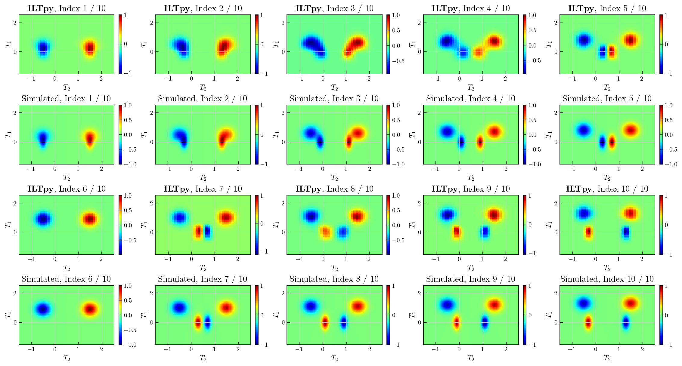
From the plots above, we see that all the components in simulated distributions are extracted at the correct positions (T1 and T2 constants) and signs after the inversion. Due to noise, the distributions from ILT are broader than the simulated distributions.
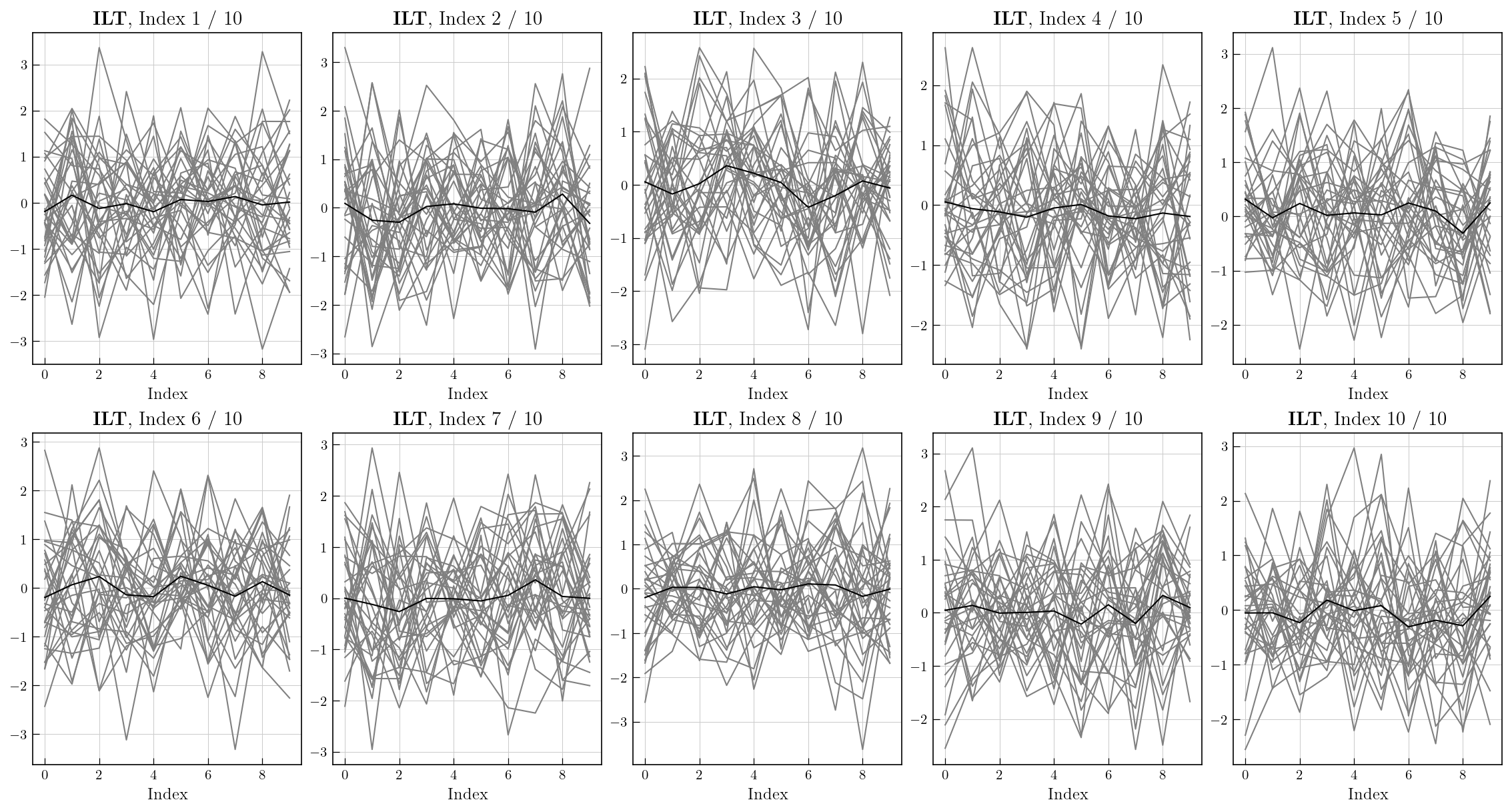
Below we plot the residuals, which should be random and devoid of systematic features for a compatible kernel and successful inversion.
[13]:
fig, axes = plt.subplots(2, 5, figsize=(15, 8), constrained_layout=True)

axes = axes.flatten()

for idx in range(10):
    ax = axes[idx]
    im = ax.plot(ilt_3d.residuals[idx].T,color='grey')
    ax.plot(np.mean(ilt_3d.residuals[idx].T,axis=1),color='k')
    ax.set_title(r"$\mathbf{ILT}$"+f", Index {idx+1} / 10")
    ax.set_xlabel("Index")