2D Data - 2D Inversion

# This file is part of ILTpy examples.
# Author : Dr. Davis Thomas Daniel
# Last updated : 25.08.2025

• This example shows how to do a 2D inversion (all dimensions are inverted) using ILTpy. Please familiarize yourself with 1D inversion with ILTpy first.

• For this example, we will first simulate some synthetic data with some postive and negative peaks.

• This example was run on a machine with Apple M1 processor (8 core CPU) and 16 GB of memory.

Imports

import iltpy as ilt
import numpy as np
import matplotlib.pyplot as plt
from iltpy.output.plotting import iltplot

print(f"ILTpy version: {ilt.__version__}")

ILTpy version: 1.0.0

Generating synthetic data

The true distribution

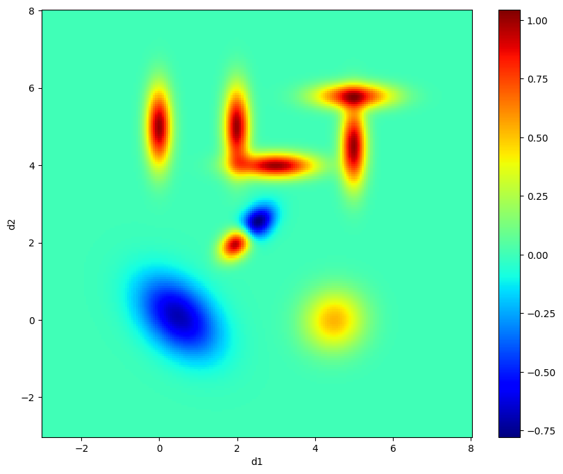
• We generate Gaussians in 2D to make a pattern which spells “ILT” along with various positive and negative peaks.

from scipy.stats import multivariate_normal
import numpy as np
import matplotlib.pyplot as plt


## Generate 2D Gaussian distributions
d1_constants = [
    0,
    2, 3,
    5, 5,
    0.5,2,2.5,4.5
]
d2_constants = [
    5,
    5, 4,
    5.8, 4.5,
    0.1,2,2.5,0
]

covariances = [
    [[0.05, 0], [0, 0.5]],
    [[0.05, 0], [0, 0.5]], [[0.5, 0], [0, 0.05]],
    [[0.5, 0], [0, 0.05]], [[0.05, 0], [0, 0.5]],
    [[0.5, -0.2], [-0.2, 0.5]],
    [[0.08, 0.03], [0.03, 0.08]],
    [[0.1, 0.04], [0.04, 0.1]],
    [[0.3, -0.01], [0.01, 0.3]],
]

amplitudes = [
    1,
    1, 1,
    0.85, 1,
    -2, 0.5, -0.5,1
]

dim1 = np.linspace(-3, 8, 200)
dim2 = np.linspace(-3, 8, 200)
X, Y = np.meshgrid(dim1, dim2)
pos = np.dstack((X, Y))

dist2d = np.zeros_like(X)
for mean, cov, amp in zip(zip(d1_constants, d2_constants), covariances, amplitudes):
    rv = multivariate_normal(mean, cov)
    dist2d += amp * rv.pdf(pos)

Visualize the true distribution

# Plot the generated dataset
plt.figure(figsize=(10, 8))
plt.pcolor(X, Y, dist2d, cmap='jet')
plt.colorbar()
plt.xlabel('d1')
plt.ylabel('d2')

Text(0, 0.5, 'd2')

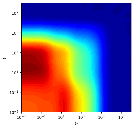
Generate time-domain data

## Time domain data :
#timing
t_syn1 = np.logspace(-3,8,32).reshape((-1,1))
t_syn2 = np.logspace(-3,8,32).reshape((-1,1))

# kernel matrix
K_matrix1 = ilt.Exponential().kernel(t_syn1,10**dim1)
K_matrix2 = ilt.Exponential().kernel(t_syn2,10**dim2)

snr = 10
syn_data_2D = snr * K_matrix1 @ dist2d @ K_matrix2.T

## add noise
np.random.seed(2505)
syn_data_2D += np.random.randn(len(t_syn1),len(t_syn2))

Visualize time-domain data

fig,ax = plt.subplots(figsize=(5,5))
ax.contourf(t_syn2.flatten(),t_syn1.flatten(),syn_data_2D,levels=70,cmap='jet')
ax.set_ylabel('t'+r'$_1$')
ax.set_xlabel('t'+r'$_2$')

plt.xscale('log')
plt.yscale('log')
plt.savefig('test.png',dpi=500)

Iltpy Workflow

Load data

# load data into an IltData object by specifying the data and the input sampling arrays
ilt_2d = ilt.iltload(data=syn_data_2D,t=[t_syn1,t_syn2])

Initialize

tau = [np.logspace(-3,8,80),np.logspace(-3,8,80)] # define output sampling for ILT

# Here with alt_g = 6, we use a different variation of the algorithm, whcih is faster in cases where all dimensions are inverted.
ilt_2d.init(tau,kernel=[ilt.Exponential(),ilt.Exponential()],verbose=1,parameters={'alt_g':6})

Initializing...
Reading fit parameters...
Setting fit parameters...
Initializing fit parameters...
Initializing kernel matrices...
Initializing regularization matrices...
Initialization took 0.035 seconds.

Invert

ilt_2d.invert()

Starting iterations ...

100%|██████████| 100/100 [02:10<00:00,  1.30s/it]

Done.

Plot results

_=iltplot(ilt_2d)

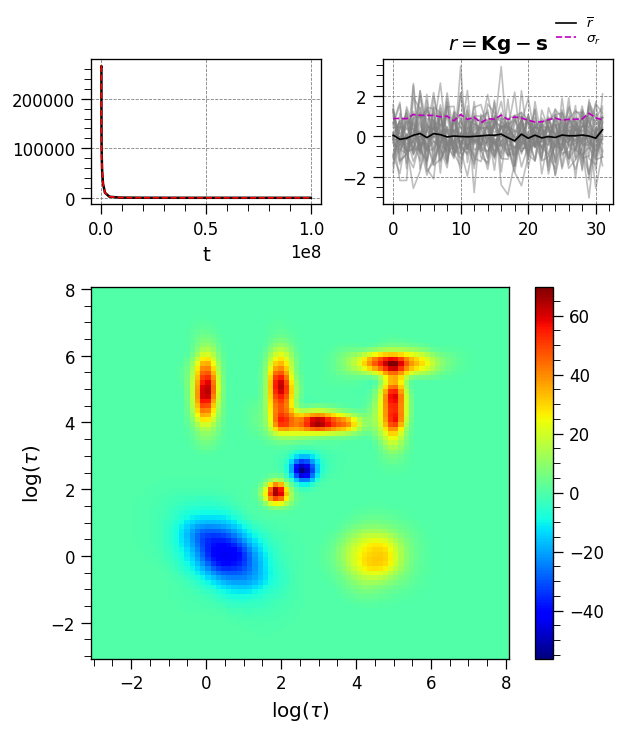
• From the plots above, we see that all the components in simulated distribution are extracted at the correct positions and shapes. Furthermore, the residuals are random and devoid of any systematic features, suggesting a successful inversion.