Inversion recovery

# This file is part of ILTpy examples.
# Author : Dr. Davis Thomas Daniel
# Last updated : 25.08.2025

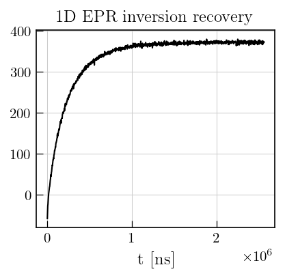
This example shows steps to invert an EPR inversion recovery dataset using ILTpy. Data is loaded using numpy arrays.

Importing iltpy and loading data

# import iltpy
import iltpy as ilt

# other libraries for handling data, plotting
import numpy as np
import matplotlib.pyplot as plt
import matplotlib.gridspec as gridspec
plt.style.use('../../../examples/latex_style.mplstyle')

print(f"ILTpy version: {ilt.__version__}")

ILTpy version: 1.0.0

# Load data using numpy arrays
data_EPR = np.loadtxt('../../../examples/EPR/inversion_recovery/data.txt') # intensity
t_EPR = np.loadtxt('../../../examples/EPR/inversion_recovery/dim1.txt') # time

coalIR = ilt.iltload(data=data_EPR,t=t_EPR)

Note

Alternatively, data and the sampling vector can be loaded from from text files directly by following a specific naming scheme for files.

For TXT data types, iltload looks for files named data.txt and dimN.txt files, where N is the number of dimensions. In this example, the data is stored as data.txt and the delays used during the inversion recovery experiment is stored as dim1.txt. The required folder structure and naming scheme is shown below.

examples/1d_epr_t1_coal/
├── data.txt
└── dim1.txt

Then, the folderpath can be given to iltload.

coalIR = ilt.iltload('../../../examples/1d_epr_t1_coal')

# Plot the raw data
fig,ax = plt.subplots(figsize=(3,2.5))
ax.plot(coalIR.t[0].flatten(),coalIR.data,'k')
plt.xlabel('t [ns]')
a1 = plt.title('1D EPR inversion recovery',size=12)

Data preparation

# Set noise variance to 1.
## estimate noise level using some points at the end of inversion recovery trace
noise_lvl  = np.std(coalIR.data[900:])

# Scale the data with the noise level
coalIR.data = coalIR.data/noise_lvl

Initialization and inversion

# define output sampling
tau = np.logspace(0,8.5,100)

# Initialize the IltData object
coalIR.init(tau=tau,kernel=ilt.Exponential())

# Invert
coalIR.invert()

Starting iterations ...

100%|██████████| 100/100 [00:00<00:00, 693.67it/s]

Done.

Plotting results

fig = plt.figure(figsize=(5, 5))
gs = gridspec.GridSpec(2, 2, width_ratios=[1, 1])

ax0 = fig.add_subplot(gs[0])
ax1 = fig.add_subplot(gs[1])
ax2 = fig.add_subplot(gs[1,0:])

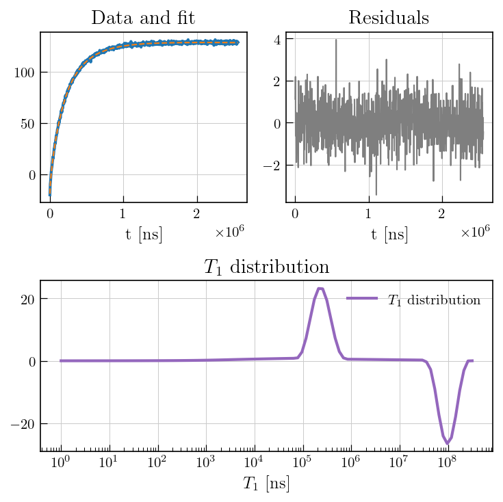
# data and fit
ax0.plot(coalIR.t[0].flatten(), coalIR.data, color='#1f77b4', label='Exp.', linewidth=2)
ax0.plot(coalIR.t[0].flatten(), coalIR.fit, color='#ff7f0e', linestyle='dashed', label='Fit')
ax0.set_xlabel('t [ns]')
ax0.set_title('Data and fit')

# residuals
ax1.plot(coalIR.t[0].flatten(), coalIR.residuals, color='#7f7f7f')
ax1.set_title('Residuals')
ax1.set_xlabel('t [ns]')

# Distribution
ax2.semilogx(coalIR.tau[0].flatten(), -coalIR.g, color='#9467bd', label=r'$T_1$'+' distribution',linewidth=2)
ax2.set_title(r'$T_1$'+' distribution')
ax2.set_xlabel(r'$T_1$'+' [ns]')
ax2.legend()

plt.tight_layout()
plt.show()

Note

• Inversion recovery curves may exhibit non-zero baselines, which may be interpreted by the algorithm as a slow relaxing component. This artefact manifests in the obtained relaxation distribution as peak with a long relaxation time constant as seen in the plot above at \(10^8\) ns. This baseline artefact can be removed by setting the sb parameter during initialization to True. See next example for usage.

• Since it is an inversion recovery, the negative of g is plotted. If the residuals do not indicate any systematic features, the chosen kernel is compatible.

Appendix : Baseline artefact

# We can test that the baseline feature is an artefact by increasing the maximum output sampling limit and checking if the feature shifts.

from copy import deepcopy

coalIR2 = deepcopy(coalIR)

# change the upper limit of output sampling
tau2 = np.logspace(0,9,100)

# initialize
coalIR2.init(tau=tau2,kernel=ilt.Exponential())

coalIR2.invert()

Starting iterations ...

100%|██████████| 100/100 [00:00<00:00, 967.83it/s]

Done.

np.log10(max(tau))

np.float64(8.5)

fig,ax = plt.subplots(figsize=(8, 3))

ax.semilogx(coalIR.tau[0].flatten(), -coalIR.g, color='#9467bd', label=r'$max(\tau) = 10^{8.5}$',linewidth=2)
ax.semilogx(coalIR2.tau[0].flatten(), -coalIR2.g, color="#254ade", label=r'$max(\tau) = 10^{9}$',linewidth=2)
ax.set_xlabel(r'$T_1$'+' [ns]')

ax.legend()

<matplotlib.legend.Legend at 0x12120f250>

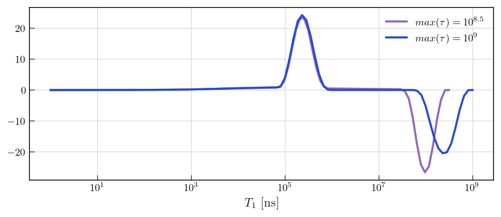
Note

• Notice that the artefact shifts with higher output sampling limit, but the real feature remains the same.