EPR : ILT without baseline artefact
[1]:
# This file is part of ILTpy examples.
# Author : Dr. Davis Thomas Daniel
# Last updated : 07.02.2026
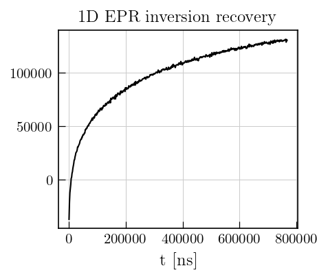
This example shows the steps to invert an inversion recovery dataset without a baseline artefact in the resulting distribution.
It is recommended to familiarize yourself with the first example in the EPR section before continuing.
The sample is a mixture of the nitroxide radical, TEMPO and carbon black in a 1:2 ratio. This dataset is taken from : https://doi.org/10.1039/D3CP00378G.
The recovery trace is stored in a file named data.txt and delays are stored in dim1.txt. Note that while reading directly from text files, a specific file naming scheme (see documentation) must be followed.
Imports
[2]:
# import iltpy
import iltpy as ilt

# other libraries for handling data, plotting
import numpy as np
import matplotlib.pyplot as plt
from iltpy.output.plotting import iltplot
print(f"ILTpy version: {ilt.__version__}")
ILTpy version: 1.1.0
Loading data from a path
[3]:
# Load data
tmspIR = ilt.iltload(data_path='../../../examples/EPR/ilt_without_baseline_artifact')
[4]:
# Plot the raw data
fig,ax = plt.subplots(figsize=(4,3.5))
ax.plot(tmspIR.t[0].flatten(),tmspIR.data,'k')
plt.xlabel('t [ns]')
a1 = plt.title('1D EPR inversion recovery',size=12)
Data preparation
For this dataset, the noise level is estimated by fitting a straight line to some points at the end of the recovery trace.
[5]:
## Fit a straight line to the end of data
x,y = tmspIR.t[0][412:],tmspIR.data[412:]
m,b = np.polyfit(x, y, 1) # fitting
noise = tmspIR.data[412:]-m*x+b # subtract the fit
noise_level = np.std(noise)

## scale data by the noise level to set the noise variance to unity
tmspIR.data = tmspIR.data/noise_level
Initialization and inversion
[6]:
## Initialize with a user-defined tau and kernel
tau = np.logspace(-7,30,800)
tmspIR.init(tau,kernel=ilt.Exponential())

tmspIR.invert()
Starting iterations ...
100%|██████████| 100/100 [00:01<00:00, 95.85it/s, Convergence=1.25e-03]
Done.
Plotting results
Results can also be plotted quickly using ILTpy’s in-built iltplot
[7]:
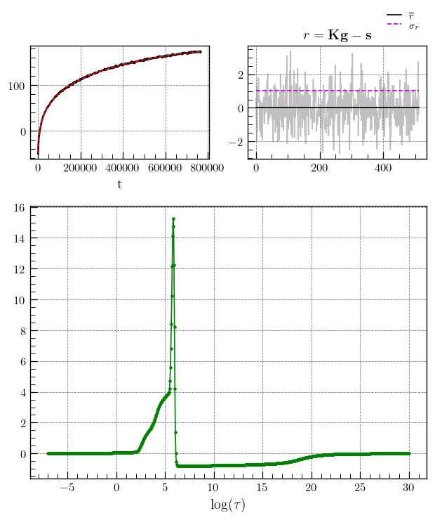
_=iltplot(tmspIR,negative_g=True)
Note
Inversion recovery curves may exhibit non-zero baselines, which may be interpreted by the algorithm as a slow relaxing component.
This artefact manifests in the obtained relaxation distribution as a negative peak with a long relaxation time constant, as seen above.
This baseline artefact is avoided by adding an additional data point to the time trace and fitting the baseline as a single value.
In ILTpy, this can be achieved by setting the parameter ‘sb’ to True.
Since an additional data point is added, the resulting distribution also contains an extra point.
[8]:
## Initialize again with parameter 'sb' set to True
tau = np.logspace(-7,30,800)
tmspIR.init(tau,kernel=ilt.Exponential(),parameters={'sb':True})

tmspIR.invert()
Starting iterations ...
100%|██████████| 100/100 [00:01<00:00, 94.39it/s, Convergence=1.07e-04]
Done.
[9]:
tmspIR.g.shape # one extra point in the resulting distribution, iltplot accounts for this while plotting.
[9]:
(801,)
[10]:
_=iltplot(tmspIR,negative_g=True)
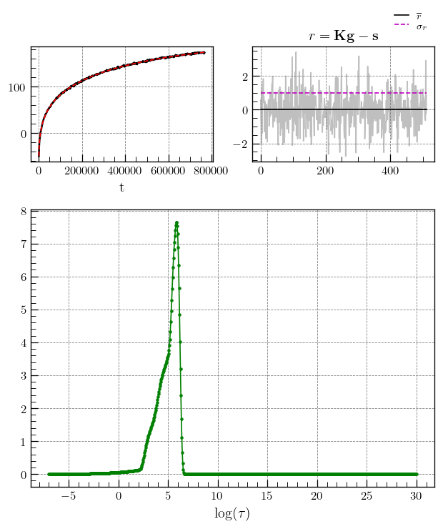
Three resolved relaxation components, corresponding to different contact qualities of nitroxide/carbon black are observed in the \(T_1\) distribution.