Field resolved inversion recovery (2D)
[1]:
# This file is part of ILTpy examples.
# Author : Dr. Davis Thomas Daniel
# Last updated : 16.02.2026
2D EPR : \(T_1\) Field dependence
This example shows steps to invert a 2D EPR dataset from a magnetic field resolved \(T_1\) experiment.
It is recommended to familiarize yourself with the first example in the EPR section before continuing.
The sample is poly(TEMPO) methacrylate mixed with carbon black. The data is loaded from numpy arrays.
Note
In this example, only the first dimension (IR delays) is inverted while both dimensions are regularized. The same applies for NMR experiments.
For the dimension which is not inverted but regularized, the input sampling vector is internally chosen as an array with unity spacing, having the same number of elements as the size of that dimension.
For majority of the cases, this is a suitable choice. However, depending on how densely the data was sampled, the input sampling vector may need adjustment.
User-defined input sampling vector in the dimension which is not inverted can be provided by passing the parameter
dim_ndimduring initialization.Similar to 1D Inversion recovery datasets, negative features at very long relaxation times arise from the baseline artefact. For 2D datasets, an example of removing the baseline artefact is shown in advanced examples.
Importing iltpy and loading data
[2]:
# import iltpy
import iltpy as ilt

# other libraries for handling data, plotting
import numpy as np
import matplotlib.pyplot as plt

print(f"ILTpy version: {ilt.__version__}")
ILTpy version: 1.1.0
[3]:
# Load data
dataIR = np.loadtxt('../../../examples/EPR/field_resolved_inversion_recovery/data.txt')
dim1 = np.loadtxt('../../../examples/EPR/field_resolved_inversion_recovery/dim1.txt') # IR delays

# input sampling vectors for the first dimension is dim 1, for second dimension which is not inverted (magnetic field), an input sampling vector is chosen internally
ptma_t1 = ilt.iltload(data=dataIR,t=dim1)

# 512 points in inversion trace and 24 field points, dimension to be inverted should always be the first.
print(f'Data size : {ptma_t1.data.shape}')
Data size : (512, 24)
Note
In case of 2D datasets, where only the first dimension is inverted, the dimension which is inverted must be the first. Data may need to be transposed accordingly.
[4]:
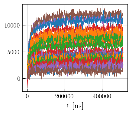
# Plot the recovery dimension
fig,ax = plt.subplots(figsize=(5,4.5))
ax.plot(ptma_t1.t[0].flatten(),ptma_t1.data)
_=ax.set_xlabel('t [ns]')
Data preparation
[5]:
## Estimate noise level by fitting a straight line to a few points at the end of inversion recovery
x,y = ptma_t1.t[0].flatten()[412:],ptma_t1.data[412:,0] # select some points from the end of the data
m,b = np.polyfit(x,y,1) # fitting a straight line to this regions
ptma_t1.data = ptma_t1.data/np.std(ptma_t1.data[412:,0]-m*x+b) # subtracting the fit
Initialization and inversion
[6]:
## intialize with user defined tau
tau = np.logspace(-7,30,251)

ptma_t1.init(tau,kernel=ilt.Exponential())

ptma_t1.invert()
Starting iterations ...
100%|██████████| 100/100 [01:51<00:00, 1.11s/it, Convergence=8.24e-04]
Done.
Plotting results
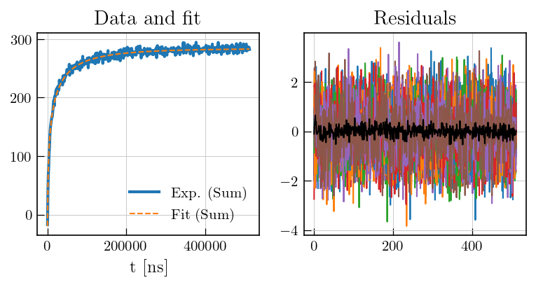
Plot fit and residuals
[7]:
# plot the fit and residuals

fig,ax = plt.subplots(figsize=(10,3.5),ncols=2)
ax[0].plot(ptma_t1.t[0].flatten(),ptma_t1.data.sum(axis=1),color='#1f77b4', label='Exp. (Sum)', linewidth=2)
ax[0].plot(ptma_t1.t[0].flatten(),ptma_t1.fit.sum(axis=1), color='#ff7f0e', linestyle='dashed', label='Fit (Sum)')
ax[0].set_xlabel('t [ns]')
ax[0].set_title('Data and fit')
ax[0].legend()


ax[1].plot(ptma_t1.residuals)
ax[1].plot(ptma_t1.residuals.mean(axis=1),color='black') # mean of residuals
a1 = ax[1].set_title('Residuals')
Plot distribution
[15]:
field_vals = np.array([3460.    , 3463.47826087, 3466.95652174, 3470.43478261,
        3473.91304348, 3477.39130435, 3480.86956522, 3484.34782609,
        3487.82608696, 3491.30434783, 3494.7826087 , 3498.26086957,
        3501.73913043, 3505.2173913 , 3508.69565217, 3512.17391304,
        3515.65217391, 3519.13043478, 3522.60869565, 3526.08695652,
        3529.56521739, 3533.04347826, 3536.52173913, 3540.        ])
fig,ax = plt.subplots(figsize=(7,5))
c = ax.contourf(field_vals,ptma_t1.tau[0].flatten()/1000,-ptma_t1.g,levels=80,cmap='jet')
ax.set_yscale('log')
ax.set_ylabel(r'$T_{1}\mathrm{[\mu s]}$')
ax.set_xlabel('Magnetic Field [mT]')
_=plt.colorbar(c)
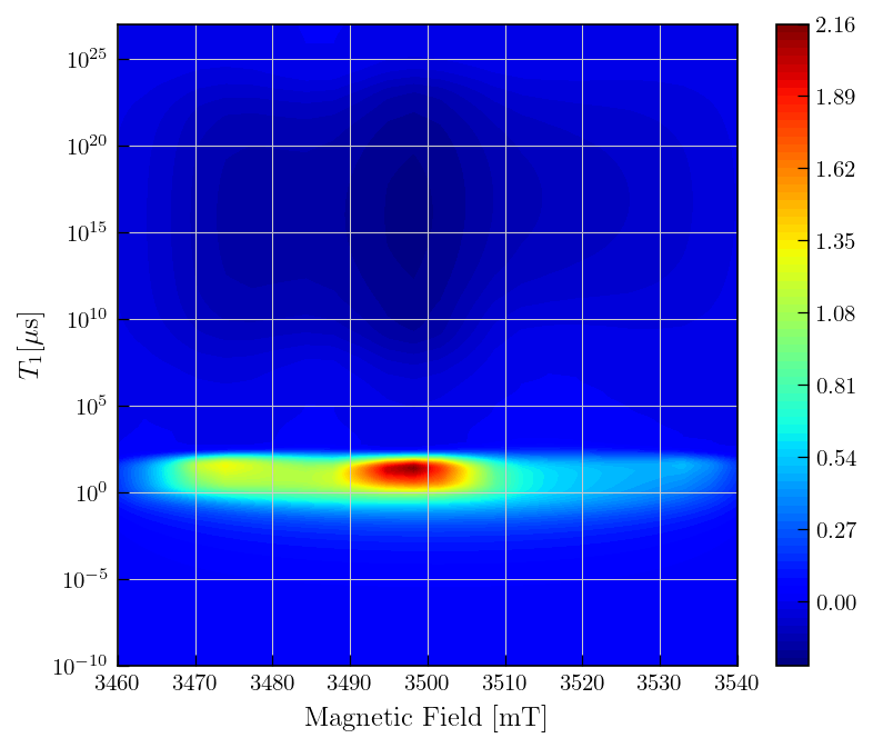
Note
Inversion recovery curves may exhibit non-zero baselines, which may be interpreted by the algorithm as a slow relaxing component.
This artefact manifests in the obtained relaxation distribution as a negative peak with a long relaxation time constant, as seen above.
You can separate this artifact from the real feature by defining a tau vector which has its maximum farther away from the feature of interest.
This artifact can also be removed by using the
sbparameter as shown in other inversion recovery examples. (see an example)