Hahn echo decay

# This file is part of ILTpy examples.
# Author : Dr. Davis Thomas Daniel
# Last updated : 25.08.2025

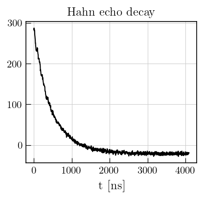
This example shows steps to invert an EPR echo decay dataset using ILTpy to extract phase memory time constants, \(T_m\) from an echo decay.

Imports

# import iltpy
import iltpy as ilt

# other libraries for handling data, plotting
import numpy as np
import matplotlib.pyplot as plt
import matplotlib.gridspec as gridspec
plt.style.use('../../../examples/latex_style.mplstyle') # plot style configuration

print(f"ILTpy version: {ilt.__version__}")

ILTpy version: 1.0.0

Data preparation

Load data from text files into numpy arrays

# Load data
data_coal = np.loadtxt('../../../examples/EPR/hahn_echo_decay/hahn_echo_decay_data.txt') # decay trace, intensity
t_coal = np.loadtxt('../../../examples/EPR/hahn_echo_decay/hahn_echo_decay_delays.txt') # tau delays

# Plot the raw data
fig,ax = plt.subplots(figsize=(3,2.5))
ax.plot(t_coal,data_coal,'k')
plt.xlabel('t [ns]')
a1 = plt.title('Hahn echo decay',size=12)

Set noise variance to unity

# Set noise variance to 1.
## estimate noise level using some points at the end of inversion recovery trace
noise_lvl  = np.std(data_coal[900:])

# Scale the data with the noise level
data_coal = data_coal/noise_lvl

ILTpy workflow

Load data

coalTM = ilt.iltload(data=data_coal,t=t_coal)

Initialization and inversion

# Initialize the IltData object
tau = np.logspace(0,6,100)
coalTM.init(tau,kernel=ilt.Exponential())

# Invert
coalTM.invert()

Starting iterations ...

100%|██████████| 100/100 [00:00<00:00, 763.87it/s]

Done.

Plot the results

fig = plt.figure(figsize=(5, 5))
gs = gridspec.GridSpec(2, 2, width_ratios=[1, 1])

ax0 = fig.add_subplot(gs[0])
ax1 = fig.add_subplot(gs[1])
ax2 = fig.add_subplot(gs[1,0:])

# data and fit
ax0.plot(coalTM.t[0].flatten(), coalTM.data, color='#1f77b4', label='Exp.', linewidth=2)
ax0.plot(coalTM.t[0].flatten(), coalTM.fit, color='#ff7f0e', linestyle='dashed', label='Fit')
ax0.set_xlabel('t [ns]')
ax0.set_title('Data and fit')

# residuals
ax1.plot(coalTM.t[0].flatten(), coalTM.residuals, color='#7f7f7f')
ax1.set_title('Residuals')
ax1.set_xlabel('t [ns]')

# Distribution
ax2.semilogx(coalTM.tau[0].flatten(), coalTM.g, color='#9467bd', label=r'$T_m$'+' distribution',linewidth=2)
ax2.set_title(r'$T_m$'+' distribution')
ax2.set_xlabel(r'$T_m$'+' [ns]')
ax2.legend()

plt.tight_layout()
plt.show()

Note

• Oscillations in residuals arise from Electron spin echo envelope modulation (ESEEM).

• See advanced examples for treating data with pronounced ESEEM oscillations.