Inversion recovery experiment

# This file is part of ILTpy examples.
# Author : Dr. Davis Thomas Daniel
# Last updated : 16.02.2026

• This example shows steps to invert a NMR inversion recovery dataset.

• The data was acquired using sample of tetra-\(\mathrm{Li}_{7}\mathrm{SiPS}_{8}\) at a magic angle spinning frequency of 20 KHz and \(\nu_{31_{\mathrm{P}}}\) = 323 MHz.

Imports

# import iltpy
import iltpy as ilt

# other libraries for handling data, plotting
import numpy as np
import matplotlib.pyplot as plt

print(f"ILTpy version: {ilt.__version__}")

ILTpy version: 1.1.0

• Load already processed data (i.e. after Fourier transformation and routine NMR processing steps)

Data preparation

Load data from text files into numpy arrays

# load data from text files into numpy arrays
lsps_data = np.loadtxt('../../../examples/NMR/inversion_recovery/data.txt')
lsps_vdlist = np.loadtxt('../../../examples/NMR/inversion_recovery/dim1.txt')
print(f'Original data size : {lsps_data.shape}')

Original data size : (15, 65536)

Data reduction

Note

In case of pseudo-2D inversions, such as pseudo-2D NMR datasets, only the first dimension is inverted but both dimensions are regularized. In this case, number of points in the uninverted dimension influences the computation time and memory requirements. Qualitatively, the number of data points along the spectral dimension (i.e., the dimension that is regularized but not inverted) should be sufficient to ensure that each resonance peak is sampled with greater density than its full width at half maximum (FWHM). With large number of points, the computation time and memory requirements also increase. Note that the sampling array for the non-inverted but regularized dimension may require adjustment depending on sampling density of the original data.

# Reduce data by a moving mean
lsps_data_red = np.reshape(lsps_data,(15,1024,64))
lsps_data_red = np.squeeze(np.mean(lsps_data_red,axis=2))
print(f'Reduced data size : {lsps_data_red.shape}')

Reduced data size : (15, 1024)

• The data consists of 15 recovery delays and for each delay, a spectrum of 65536 points.

• To reduce computational demands of the inversion, the data is reduced.

• The data was reduced to (15,1024) by moving mean.

• Alternatively, number of points can be reduced by decreasing the sampling.

lsps_data_red = lsps_data[:,0:65536:65] # selects spectrum points with a spacing of 65 for each delay

Set noise variance to unity

Note

For inversion, ILTpy expects data which has Gaussian identically distributed noise with a variance of 1. Most experimental datasets need to be scaled with the noise level in order to fulfill this condition. A common practice in case of magnetic resonance data is to select a region with a flat baseline and with only noise. The data is then scaled with the standard deviation of data points in this region.

## Setting noise variance to unity

# To estimate noise, select a region with no signal
fig,ax = plt.subplots(figsize=(8,3.5),ncols=2)
ax[0].plot(lsps_data_red[-1])
ax[1].plot(lsps_data_red[-1][220:350])
ax[0].set_title('NMR spectrum')
ax[1].set_title('Noise region')

Text(0.5, 1.0, 'Noise region')

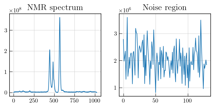
Note

The noise should be estimated from a region with random noise and no systematic features. In case of spectra with distorted baselines, the noise region can be obtained by doing an additional baseline correction for the corresponding region and then estimating the noise level.

# and calculate the noise level
noise_lvl = np.std(lsps_data_red[-1][220:350])

# scale data with the noise_lvl
lsps_data_red = lsps_data_red/noise_lvl

ILTpy workflow

Load data

lspsILT = ilt.iltload(data=lsps_data_red,t=lsps_vdlist)

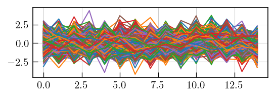
# Plot the data
fig,ax = plt.subplots(figsize=(5,3.5))
a = ax.plot(lspsILT.data.flatten())

Initialization and inversion

# Intialization
tau = np.logspace(-2,5,100) ##user-defined tau
lspsILT.init(tau,kernel=ilt.Exponential())

# Inversion
lspsILT.invert()

Starting iterations ...

100%|██████████| 100/100 [05:27<00:00,  3.28s/it, Convergence=8.71e-04]

Done.

Plot the results

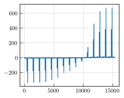
# In case of a compatible kernel, the residuals should be random, devoid of systematic features.
# check residuals for systematic features
fig,ax = plt.subplots(figsize=(5,1.2))
a = ax.plot(lspsILT.residuals)

# load the ppm axis for plotting

ppm_axis = np.loadtxt('../../../examples/NMR/inversion_recovery/chemical_shift_axis.txt')
ppm_axis = np.reshape(ppm_axis,(1024,64))
ppm_axis = np.mean(ppm_axis,axis=1)

# Generate x, y, z values from the lspsILT object
# use the ppm axis for plotting

x, y = ppm_axis[300:700], lspsILT.tau[0].flatten()
Z = -lspsILT.g[:,300:700]

fig,ax = plt.subplots()
a = ax.contourf(x,np.log10(y),Z,cmap='jet',levels=150)
ax.set_xlabel(r"$^{31}\mathrm{P}$"+' chemical shift [ppm]')
ax.set_ylabel('log('+r'$T_{1})$')

plt.colorbar(a)

<matplotlib.colorbar.Colorbar at 0x133a26270>

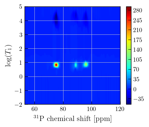
Note

• Inversion recovery curves may exhibit non-zero baselines, which may be interpreted by the algorithm as a slow relaxing component (the negative peaks around \(10^{4}\)).

• This artefact manifests in the obtained relaxation distribution as a negative peak with a long relaxation time constant, as seen above.

• The artefact may be separated from the features of interest by choosing a tau with a higher maximum value.

• The artefact can also be removed by using the static baseline feature as shown below using the sb parameter (available from v.1.1.0)

Static baseline

tau = np.logspace(-2,5,100)
lspsILT.init(tau,kernel=ilt.Exponential(),parameters={"sb":[True,False]}) # we only want the static baseline feature to be applied in the relaxation dimension, not the spectral dimension
lspsILT.invert()

Starting iterations ...

100%|██████████| 100/100 [05:36<00:00,  3.37s/it, Convergence=3.41e-04]

Done.

fig, ax = plt.subplots(figsize=(5, 5))
g = ax.contourf(
    ppm_axis[350:650],
    lspsILT.tau[0].flatten(),
    np.negative(lspsILT.g[:-1, 350:650]),
    cmap="jet",levels=150
)  # since we use sb as a parameter, an extra point is added to the distribution, we skip this point while plotting since it only fits the baseline.
ax.set_yscale("log")
ax.set_ylabel(r"$T_{1}$" + " [s]")
ax.set_xlabel(r"$^{31}\mathrm{P}$" + " chemical shift [ppm]")
ax.invert_xaxis()
# fig.colorbar(g,ax)
ax.grid()

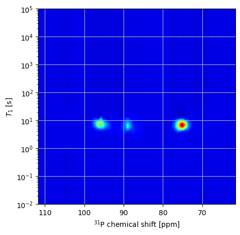
Note

• By specifiying sb=[True, False], we fit the baseline in the inversion recovery dimension using a single point and it no longer appears as an artefact in the resulting distribution.

• Note that the actual features do not change their position.

• It is recommended to review the distribution both with and without the static baseline feature enabled and compare them to ensure the actual features are accurately reproduced in the version where the static baseline is active.