Inversion recovery-CPMG experiment (2D ILT)

# This file is part of ILTpy examples.
# Author : Dr. Davis Thomas Daniel
# Last updated : 16.02.2026

• This example shows steps to invert a \(T_1-T_2\) correlation dataset with data compression.

• It is recommended to familiarize yourself with the first example in the NMR section before continuing.

• The same workflow may be used for other 2D inversions.

Importing iltpy and loading data

# import iltpy
import iltpy as ilt
# other libraries for handling data, plotting
import numpy as np
import matplotlib.pyplot as plt
from iltpy.output.plotting import iltplot

print(f"ILTpy version: {ilt.__version__}")

ILTpy version: 1.1.0

• Load already processed data (i.e. after Fourier transformation and routine NMR processing steps)

t1t2_corr_data = np.loadtxt('../../../examples/NMR/t1_t2_correlation_2d/t1_t2_correlation_data.txt') ## 2D data
t_recovery = np.loadtxt('../../../examples/NMR/t1_t2_correlation_2d/t_recovery.txt') ## T1 recovery delays
t_cpmg = np.loadtxt('../../../examples/NMR/t1_t2_correlation_2d/t_cpmg.txt') ## cpmg delays

t1t2_corr_data.shape,t_cpmg.shape,t_recovery.shape  # CPMG delays along axis 0 and T1 recovery delays along axis 1

((256, 22), (256,), (22,))

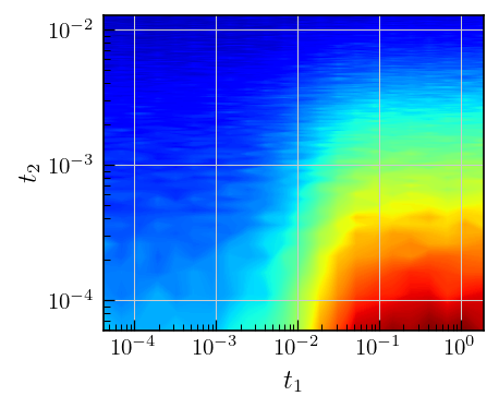
# Plot the data
fig,ax = plt.subplots(figsize=(5,4.5))
a = ax.contourf(t_recovery,t_cpmg,t1t2_corr_data,cmap='jet',levels=500)
ax.set_yscale('log')
ax.set_xscale('log')
ax.set_ylabel(r'$t_2$')
_=ax.set_xlabel(r'$t_1$')

Data preparation

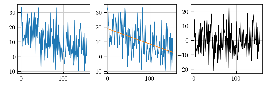
# noise estimation by baseline correction
fig,ax = plt.subplots(ncols=3,figsize=(10,3))
## select a noise region
ax[0].plot(t1t2_corr_data[100:,-1])

## fit a straight line
y = t1t2_corr_data[100:,-1]
x = np.arange(0,len(y))
coeff = np.polyfit(x,y,deg=1)
y_fit = np.polyval(coeff,x=x)

# fit of the noise region
ax[1].plot(x,y)
ax[1].plot(x,y_fit)

# fit of residuals
residuals = y-y_fit
_=ax[2].plot(x,residuals,'k')

print(f'Standard deviation : {np.std(residuals)}')

Standard deviation : 8.705347107839648

# Set noise variance to unity
t1t2_corr_data = t1t2_corr_data/8.705347107839648

Iltpy Workflow

Load data

# load data into an IltData object.
t1t2ILT = ilt.iltload(data=t1t2_corr_data,t=[t_cpmg,t_recovery])

t1t2ILT.data

array([[ 5.29039071e+01,  5.54526280e+01,  5.45551911e+01, ...,
         1.50889063e+01,  1.46252305e+01,  1.64081386e+01],
       [ 5.05885199e+01,  4.96372367e+01,  4.76688584e+01, ...,
         1.29081345e+01,  1.15859108e+01,  1.28213823e+01],
       [ 4.54551806e+01,  4.54821037e+01,  4.64902245e+01, ...,
         1.19179625e+01,  1.22410398e+01,  1.19718087e+01],
       ...,
       [ 1.06196704e+00,  9.48291692e-01,  2.00726727e+00, ...,
         1.05299267e+00,  2.14786572e+00, -5.23504877e-01],
       [ 2.57564400e+00,  1.13974490e+00,  1.19658258e-02, ...,
        -5.32479246e-01,  1.67521561e-01,  1.43889055e+00],
       [ 3.20684130e+00,  2.94359314e+00,  2.77906303e+00, ...,
         1.24743734e+00, -5.86325462e-01,  7.17949546e-02]],
      shape=(256, 22))

Initialization and inversion

• To reduce computational needs, data can compressed using singular value decomposition along both dimensions.

• During initialization, set the compress parameter to True for both dimensions.

• s specifies the number of the singular values.

• For 2D inversions, another variation of the algorithm which performs faster, is used and is specified by alt_g = 8.

# define the parameters as a dict
p_dict = {'compress':[True,True],'s':[12,22],'alt_g':8}
# define tau for both dimensions
tau = [np.logspace(-5,-1,130),np.logspace(-5,5,130)]
# initialize with exponential kernel in both dimensions
t1t2ILT.init(tau,kernel=[ilt.Exponential(),ilt.Exponential()],parameters=p_dict,verbose=2)

Initializing...
Reading fit parameters...
Setting fit parameters...
Initializing fit parameters...
Initializing kernel matrices...
    Initializing kernel matrix in dimension 0...
    Initializing kernel matrix in dimension 1...
    Kernel initialization done.
Initializing regularization matrices...
   Calculating constant, regularization matrices...
   Calculating diagonal matrices...
   Calculating amplitude regularization...
   Regularization matrices initialization done.
Initialization took 0.064 seconds.

t1t2ILT.compress

[True, True]

t1t2ILT.invert()

Starting iterations ...

100%|██████████| 100/100 [03:24<00:00,  2.05s/it, Convergence=2.41e-03]

Done.

Plot results

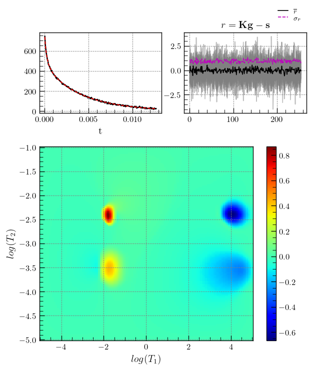
# ILTpy's plotting function iltplot is used.
# transform_g=True, which is False by default, applies the transformaton :  g = np.sign(g) * np.sqrt(np.abs(g)) and makes it easier to spot weak features.
fig,ax = iltplot(t1t2ILT,transform_g=True,negative_g=True) # for inversion recovery, the negative of g is plotted
ax[1].set_xlabel(r'$log(T_1)$')
_=ax[1].set_ylabel(r'$log(T_2)$')

Note

• Inversion recovery curves may exhibit non-zero baselines, which may be interpreted by the algorithm as a slow relaxing component (the negative peaks around \(10^{4}\)).

• This artefact manifests in the obtained relaxation distribution as a negative peak with a long relaxation time constant, as seen above.

• The artefact may be separated from the features of interest by choosing a tau with a higher maximum value.

• If the SNR is feasible, this feature can be removed by using the static baseline feature ILTpy provides, as shown below.

Static baseline

# define the parameters as a dict, we use a static baseline in the T1 dimension, set sb to True for the T1 dimension and False for the T2 dimension
p_dict = {'compress':[True,True],'s':[12,22],'alt_g':8,"sb":[False, True]}
# same tau for both dimensions as before
tau = [np.logspace(-5,-1,130),np.logspace(-5,5,130)]
# initialize with exponential kernel in both dimensions
t1t2ILT.init(tau,kernel=[ilt.Exponential(),ilt.Exponential()],parameters=p_dict,verbose=2)

Initializing...
Reading fit parameters...
Setting fit parameters...
Initializing fit parameters...
Initializing kernel matrices...
    Initializing kernel matrix in dimension 0...
    Initializing kernel matrix in dimension 1...
    Kernel initialization done.
Initializing regularization matrices...
   Calculating constant, regularization matrices...
   Calculating diagonal matrices...
   Calculating amplitude regularization...
   Regularization matrices initialization done.
Initialization took 0.039 seconds.

t1t2ILT.sb

[False, True]

t1t2ILT.invert()

Starting iterations ...

100%|██████████| 100/100 [03:28<00:00,  2.09s/it, Convergence=6.44e-04]

Done.

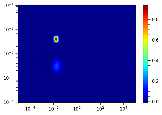
fig,ax = plt.subplots()
p = ax.pcolor(t1t2ILT.tau[1].flatten(),t1t2ILT.tau[0].flatten(),-t1t2ILT.g[:,:-1],cmap="jet") # we don't apply the transformation we applied to g before
ax.set_xscale("log")
ax.set_yscale("log")
_=plt.colorbar(p, ax=ax)

Note

• By specifiying sb=[False, True], we fit the baseline in the inversion recovery dimension using a single point and it no longer appears as an artefact in the resulting distribution.

• Note that the actual features do not change their position.

• It is recommended to review the distribution both with and without the static baseline feature enabled and compare them to ensure the actual features are accurately reproduced in the version where the static baseline is active.