Diffusion (PGSTE)
[1]:
# This file is part of ILTpy examples.
# Author : Dr. Davis Thomas Daniel
# Last updated : 16.02.206
This example shows steps to obtain diffusion constants from ILT of \({}^{1} {\mathrm{H}}\) diffusion experimental data obtained with a stimulated echo sequence.
It is recommended to familiarize yourself with the first example in the NMR section before continuing.
The data was acquired using a sample of [\(\mathrm{Pyr}_{13}\)][\(\mathrm{Tf}_{2}\mathrm{N}\)] confined to carbon black.
For more experimental details and discussion about this dataset, please refer to : https://doi.org/10.1039/C9CP02651G
Imports
[2]:
# import iltpy
import iltpy as ilt

# other libraries for handling data, plotting
import numpy as np
import matplotlib.pyplot as plt

print(f"ILTpy version: {ilt.__version__}")
ILTpy version: 1.1.0
Data preparation
Load data from text files into numpy arrays
[3]:
diff_data = np.loadtxt('../../../examples/NMR/Diffusion/diff_data.txt')
diff_B_val = np.loadtxt('../../../examples/NMR/Diffusion/diff_B_values.txt')
diff_ppm = np.loadtxt('../../../examples/NMR/Diffusion/diff_ppm_axis.txt')
Load already processed data (i.e. after Fourier transformation and routine NMR processing steps)
Load B values (usually found in diff.xml file in case of Bruker file formats)
Data reduction, setting noise variance to unity
[4]:
# Slice the data and set noise variance to unity
diff_data = diff_data[:,1850:2000]/diff_data[1,5:50].std()
ILTpy workflow
Load data
[5]:
diffILT = ilt.iltload(data=diff_data,t=diff_B_val)
print(f'Data size : {diffILT.data.shape}') # dataset is smaller in size than the orginal data
Data size : (256, 150)
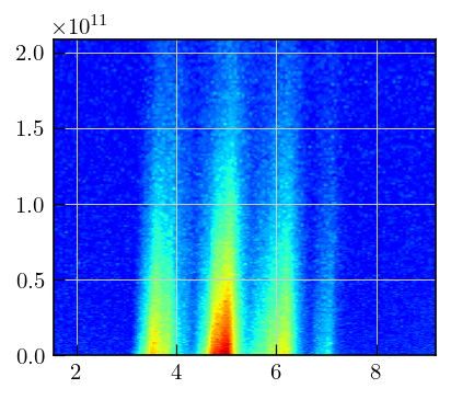
[7]:
# Plot the data
fig,ax = plt.subplots(figsize=(5,4.5))
a = ax.contourf(diff_ppm[1850:2000],diffILT.t[0].flatten(),diffILT.data,cmap='jet',levels=100)
Initialization and inversion
[8]:
# Initialization
# specify the expected range of diffusion coefficients
tau = np.logspace(-16,-8,200)
# choose diffusion kernel
diffILT.init(tau,kernel=ilt.Diffusion())

# Inversion
diffILT.invert()
Starting iterations ...
100%|██████████| 100/100 [04:44<00:00, 2.84s/it, Convergence=5.84e-04]
Done.
Plot the results
[9]:
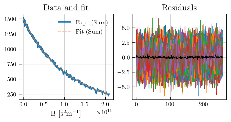
## Setting noise variance to unity

# To estimate noise, select a region with no signal
fig,ax = plt.subplots(figsize=(7,3.5),ncols=2)
ax[0].plot(diffILT.t[0].flatten(),diffILT.data.sum(axis=1),color='#1f77b4', label='Exp. (Sum)', linewidth=2)
ax[0].plot(diffILT.t[0].flatten(),diffILT.fit.sum(axis=1), color='#ff7f0e', linestyle='dashed', label='Fit (Sum)')
ax[0].set_xlabel('B ['+r'$\mathrm{s}^{2}\mathrm{m}^{-1}$'+']')
ax[0].set_title('Data and fit')
ax[0].legend()


ax[1].plot(diffILT.residuals)
ax[1].plot(diffILT.residuals.mean(axis=1),color='black') # mean of residuals
a1 = ax[1].set_title('Residuals')
[10]:
x = diff_ppm[1850:2000] # chemical shift
y = diffILT.tau[0].flatten()[50:] # output sampling vector
Z = diffILT.g[50:,:] # distribution of relaxation time constants
fig,ax = plt.subplots(figsize=(6,6))
a = ax.pcolor(x,np.log10(y),Z,cmap='jet')
ax.set_xlabel(r"$^{1}\mathrm{H}$"+' chemical shift [ppm]')
ax.set_ylabel('log(D)')

plt.colorbar(a)
[10]:
<matplotlib.colorbar.Colorbar at 0x1659102f0>
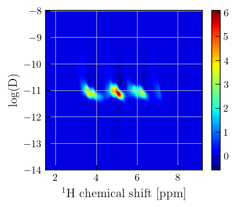
Note
Notice the negative features in the distribution close \(10^{-11}\), the validity of non-negativity constraint can be accessed by repeating the inversion with non-negativity constraint set to True and inspecting the residuals.
Repeat inversion with non-negativity constraint
[11]:
# for non-negativity constraint, set 'nn' to True
diffILT.init(tau,kernel=ilt.Diffusion(),parameters={'nn':True})

# Inversion
diffILT.invert()
Starting iterations ...
100%|██████████| 100/100 [04:45<00:00, 2.85s/it, Convergence=3.43e-04]
Done.
[12]:
x = diff_ppm[1850:2000] # chemical shift
y = diffILT.tau[0].flatten()[50:] # output sampling vector
Z = diffILT.g[50:,:] # distribution of relaxation time constants
fig,ax = plt.subplots(figsize=(6,6))
a = ax.pcolor(x,np.log10(y),Z,cmap='jet')
ax.set_xlabel(r"$^{1}\mathrm{H}$"+' chemical shift [ppm]')
ax.set_ylabel('log(D)')

plt.colorbar(a)
[12]:
<matplotlib.colorbar.Colorbar at 0x1659f92b0>

[13]:
# plot the fit and residuals
## Setting noise variance to unity

# To estimate noise, select a region with no signal
fig,ax = plt.subplots(figsize=(7,3.5),ncols=2)
ax[0].plot(diffILT.t[0].flatten(),diffILT.data.sum(axis=1),color='#1f77b4', label='Exp. (Sum)', linewidth=2)
ax[0].plot(diffILT.t[0].flatten(),diffILT.fit.sum(axis=1), color='#ff7f0e', linestyle='dashed', label='Fit (Sum)')
ax[0].set_xlabel('B ['+r'$\mathrm{m}^{2}\mathrm{s}^{-1}$'+']')
ax[0].set_title('Data and fit')


ax[1].plot(diffILT.residuals)
ax[1].plot(diffILT.residuals.mean(axis=1),color='black') # mean of residuals
a1 = ax[1].set_title('Residuals')
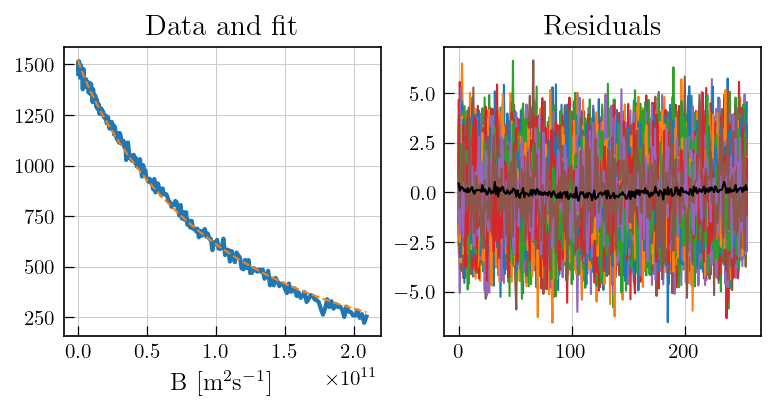
Note
The negative distribution features are supressed in the distribution which was obtained from ILT with the use of non-negativity constraint. However, the mean residuals clearly deviate from zero. This suggests that the negative features observed in the absence of non-negativity constraint, are significant and are required to fully describe the data.