CPMG (MAS, 20KHz)
[1]:
# This file is part of ILTpy examples.
# Author : Dr. Davis Thomas Daniel
# Last updated : 16.02.2026
This example shows steps to invert a NMR CPMG (Carr-Purcell-Meiboom-Gill) decay dataset.
It is recommended to familiarize yourself with the first example in the NMR section before continuing.
The data was acquired using sample of tetra-\(\mathrm{Li}_{7}\mathrm{SiPS}_{8}\) at a magic angle spinning frequency of 20 KHz and \(\nu_{31_{\mathrm{P}}}\) = 323 MHz.
Imports
[2]:
# import iltpy
import iltpy as ilt

# iltpy's plotting function
from iltpy.output.plotting import iltplot

# other libraries for handling data, plotting
import numpy as np
import matplotlib.pyplot as plt
print(f"ILTpy version: {ilt.__version__}")
ILTpy version: 1.1.0
Data preparation
The data consists of 8 echo delays and for each delay, a spectrum of 65536 points.
To reduce computational demands of the inversion, in the next step the data is reduced.
Load data from text files into numpy arrays
[3]:
cpmg_data = np.loadtxt('../../../examples/NMR/CPMG/data.txt') # spectra
cpmg_delays = np.loadtxt('../../../examples/NMR/CPMG/dim1.txt') #  cpmg echo delays

print(f"Original data size : {cpmg_data.shape}")
Original data size : (8, 65536)
Data reduction
[4]:
# Reduce data by a moving mean or by reducing the sampling
lspsCPMG_red = np.reshape(cpmg_data,(8,1024,64))
lspsCPMG_red = np.squeeze(np.mean(lspsCPMG_red,axis=2))

print(f"Reduced data size : {lspsCPMG_red.shape}")
Reduced data size : (8, 1024)
Set noise variance to unity
[8]:
## Setting noise variance to unity
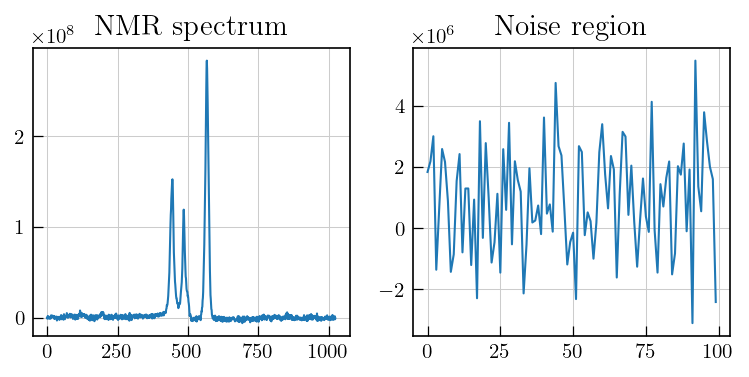
# To estimate noise, select a region with no signal
fig,ax = plt.subplots(figsize=(10,3.5),ncols=2)
ax[0].plot(lspsCPMG_red[0])
ax[1].plot(lspsCPMG_red[0][201:301])
ax[0].set_title('NMR spectrum')
ax[1].set_title('Noise region')
[8]:
Text(0.5, 1.0, 'Noise region')
[9]:
# and calculate the noise level
noise_lvl = np.std(lspsCPMG_red[-1][201:301])

# set the noise variance to unity by scaling the data
lspsCPMG_red = lspsCPMG_red/noise_lvl
Note
The noise should be estimated from a region with random noise and no systematic features. In case of spectra with distorted baselines, the noise region can be obtained by doing an additional baseline correction for the corresponding region and then estimating the noise level.
ILTpy workflow
Load data
[10]:
lspsCPMG= ilt.iltload(data=lspsCPMG_red,t=cpmg_delays) # data after reduction and setting the noise variance to unity is loaded.
In addtion to the delays provided as input, an array of unit spacing was chosen internally which matches the length of the second dimension (chemical shift axis). This can be checked by accessing the t attribute of the the
IltDataobject, as shown below.
[11]:
lspsCPMG.t
[11]:
[array([0.0040204, 0.0080408, 0.0160816, 0.0321632, 0.0643264, 0.1286528,
        0.2573056, 0.5146112]),
 array([   1,    2,    3, ..., 1022, 1023, 1024], shape=(1024,))]
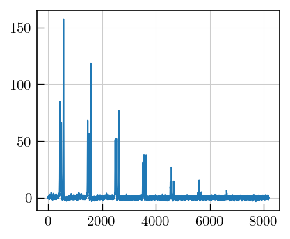
[12]:
# Plot the data
fig,ax = plt.subplots(figsize=(4,3.5))
a = ax.plot(lspsCPMG.data.flatten())
Initialization and inversion
[13]:
# Intialization
tau = np.logspace(-5.4,1.7,100) # tau array with 100 points ranging from 10^-5.4 to 10^1.7
lspsCPMG.init(tau=tau,kernel=ilt.Exponential())
[14]:
# invert
lspsCPMG.invert()
Starting iterations ...
100%|██████████| 100/100 [05:38<00:00, 3.38s/it, Convergence=4.01e-04]
Done.
Plot the results
iltplotcan also be used for 2D data.
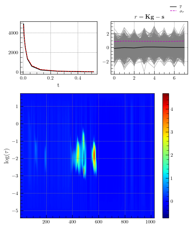
[15]:
# IltPy's plotting function iltplot is used.
# transform_g=True, which is False by default, applies the transformation :  g = np.sign(g) * np.sqrt(np.abs(g)) and makes it easier to spot weak features.
_=iltplot(lspsCPMG,transform_g=True)