Bruker NMR data, nmrglue and ILTpy

# This file is part of ILTpy examples.
# Author : Dr. Davis Thomas Daniel
# Last updated : 18.08.2025

• This example shows an ILTpy workflow involving NMR data acuqired on a Bruker spectrometer, reading and processing it using nmrglue and then ILT analysis using ILTpy.

• It is recommended to familiarize yourself with the first example in the NMR section before continuing.

• nmrglue is a python module for reading, writing, and interacting with the spectral data stored in a number of common NMR data formats. For more information see nmrglue’s documentation.

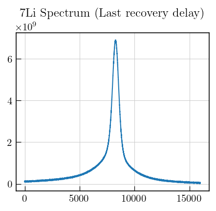
• The dataset is a 7Li inversion recovery dataset, the sample is a solid electrolyte. The measurement was done at static conditions.

Imports

import nmrglue as ng # nmrglue
import iltpy as ilt # iltpy
import numpy as np # numpy
import matplotlib.pyplot as plt # matplotlib
plt.style.use("../../../examples/latex_style.mplstyle")

print("nmrglue version: ",ng.__version__)
print("iltpy version: ",ilt.__version__)

nmrglue version:  0.11
iltpy version:  1.0.0

Read the Bruker data using nmrglue

# read in the bruker formatted data
dic, data = ng.bruker.read('../../../examples/NMR/bruker_data_IR/14') # experiment folder 9

# remove the digital filter
data = ng.bruker.remove_digital_filter(dic, data)

# process the spectrum. This may vary for your dataset, therefore, choose appropriate values.
#data = ng.proc_base.zf_size(data, 16384)   # zero fill points
data = ng.proc_base.fft(data)               # Fourier transform
data = ng.proc_base.ps(data, p0=150,p1=10)  # phase correction
data = ng.proc_base.di(data)                # discard the imaginaries

# load the vdlist (this file is usually found in the experiment folder)
vdlist = np.loadtxt("../../../examples/NMR/bruker_data_IR/14/vdlist") # vdlist contains the recovery delays in seconds.

print(f"Data shape : {data.shape}") # there are 11 recovery delays and each spectrum has 33202 points

Data shape : (11, 33202)

# calculate chemical shift axis in ppm, (Important! : Reference it appropriately for your dataset)
offset = (float(dic['acqus']['SW']) / 2) - (float(dic['acqus']['O1']) / float(dic['acqus']['BF1'])) #calculate frequency offset
start = float(dic['acqus']['SW']) - offset #calculate higher limit of ppm scale
end = -offset #calculate lower limit of ppm scale
step = float(dic['acqus']['SW']) / data.shape[1] #calculate interval
chemical_shift_ppm = np.arange(start, end, -step)

print(f"Spacing of chemical shift axis : {np.mean(np.diff(chemical_shift_ppm))}")

Spacing of chemical shift axis : -0.0060528671508279785

# The size of the first dimension (11 in this case) should match the number of delays in the vdlist
print(f"Number of delays in vdlist : {len(vdlist)}")

Number of delays in vdlist : 11

# plot the last recovery delay
fig,ax = plt.subplots()
ax.plot(data[-1][9000:25000]) # a region from the full spectrum
ax.set_title("7Li Spectrum (Last recovery delay)",fontsize=12)

Text(0.5, 1.0, '7Li Spectrum (Last recovery delay)')

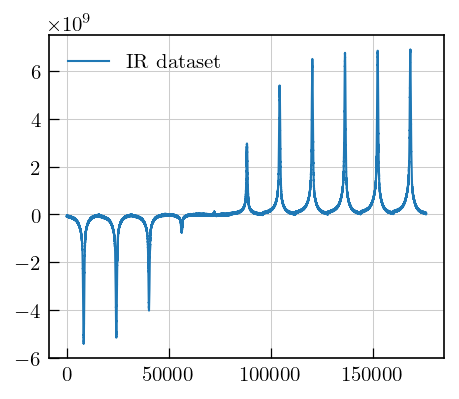
# plot the whole dataset
fig,ax = plt.subplots()
ax.plot(data[0:11,9000:25000].flatten(),label="IR dataset") # plot all spectra as a flattened array
ax.legend()

<matplotlib.legend.Legend at 0x111551be0>

Data preparation

Data reduction

# reduce the data, by reducing the sampling, this reduces the computational expense of the inversion
data_red = data.copy()
data_red = data_red[:,9000:25000:15] # we pick every 15th point from data point index 9000 to 25000

data_red.shape

(11, 1067)

Set the noise variance to unity

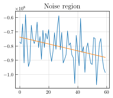
# select a region with noise, calculate standard deviation
fig,ax = plt.subplots()
ax.plot(data_red[0][10:70]) # Here, noise region from spectrum corresponding to first recovery delay is chosen
ax.set_title("Noise region")

# fit a straight line to remove background
m,b = np.polyfit(np.arange(10,70),data_red[0][10:70],deg=1)
fit = m*np.arange(10,70)+b
plt.plot(m*np.arange(10,70)+b)

print(f"SD : {np.std(data_red[0][10:70]-fit)}") # subtract the fit and calculate standard deviation of the

SD : 10240545.292070072

# scale the data with the obtained value from the previous step.

data_red = data_red/10240545.292070072

ILTpy workflow

Load the data

# provide the reduced data and the vdlist to iltpy
ir_ilt = ilt.iltload(data=data_red,t=vdlist)

Initialize and invert

# initialize by providing tau and specifying kernel
tau = np.logspace(-2.5,5,80) # output sampling vector

# specify an exponential kernel for T1, Inversion recovery
# we also specify a more closely spaced array in the non-inverted, but regularized second dimension.
ir_ilt.init(tau,kernel=ilt.Exponential(),dim_ndim=np.arange(1,1068)/150)

ir_ilt.invert()

Starting iterations ...

100%|██████████| 100/100 [04:49<00:00,  2.89s/it]

Done.

Plot the results

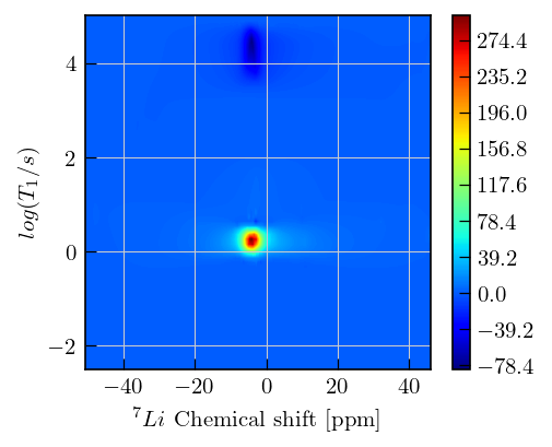
fig,ax = plt.subplots()

x = chemical_shift_ppm[9000:25000:15].flatten() # chemical shift values for the region which was inverted
y = np.log10(ir_ilt.tau[0]).flatten()           # ouput sampling vector, T1 values
dist = -ir_ilt.g                                # relaxation distribution, we plot the negative here since it is an inversion recovery dataset
c = ax.contourf(x,y,dist,cmap='jet',levels=500)

ax.set_xlabel(r'$^{7}Li$'+' Chemical shift [ppm]',fontsize=10)
ax.set_ylabel(r'$log(T_{1}/s)$',fontsize=10)
_=fig.colorbar(c, ax=ax)

# we can calculate the T1 value corresponding the the maximum intensity:

dist_max = np.max(dist)
dist_max_index = np.unravel_index(np.argmax(dist),dist.shape)
t1_max  = ir_ilt.tau[0][dist_max_index[0]]

print(f"T1 value at max : {t1_max[0]:.2f} s")

T1 value at max : 1.79 s

Note

• Inversion recovery curves may exhibit non-zero baselines, which may be interpreted by the algorithm as a slow relaxing component.

• This artefact manifests in the obtained relaxation distribution as a negative peak with a long relaxation time constant, as seen above.

• You can separate this artifact from the real feature by defining a tau vector which has its maximum farther away from the feature of interest.