The filtering file prepared in Section Optimizing the measurement configuration can now be applied to produce a new summary measurement, ideally with reduced measurement overhead to improve accuracy. This can be accomplished by providing the filter file name to scalasca -analyze via the -f option.

Attention: Before re-analyzing the application, the unfiltered summary experiment should be renamed (or removed), since scalasca -analyze will not overwrite the existing experiment directory and abort immediately.

  % mv scorep_bt_64_sum scorep_bt_64_sum.nofilt
  % scalasca -analyze -f npb-bt.filt mpiexec -n 64 ./bt.D.64
  S=C=A=N: Scalasca 2.2 runtime summarization
  S=C=A=N: ./scorep_bt_64_sum experiment archive
  S=C=A=N: Thu Jan 29 22:20:59 2015: Collect start
  mpiexec -n 64  [...]  ./bt.D.64


   NAS Parallel Benchmarks 3.3 -- BT Benchmark

   No input file inputbt.data. Using compiled defaults
   Size:  408x 408x 408
   Iterations:  250    dt:   0.0000200
   Number of active processes:    64

   Time step    1
   Time step   20
   Time step   40
   Time step   60
   Time step   80
   Time step  100
   Time step  120
   Time step  140
   Time step  160
   Time step  180
   Time step  200
   Time step  220
   Time step  240
   Time step  250
   Verification being performed for class D
   accuracy setting for epsilon =  0.1000000000000E-07
   Comparison of RMS-norms of residual
             1 0.2533188551738E+05 0.2533188551738E+05 0.1479210131727E-12
             2 0.2346393716980E+04 0.2346393716980E+04 0.8488743310506E-13
             3 0.6294554366904E+04 0.6294554366904E+04 0.3034271788588E-14
             4 0.5352565376030E+04 0.5352565376030E+04 0.8597827149538E-13
             5 0.3905864038618E+05 0.3905864038618E+05 0.6650300273080E-13
   Comparison of RMS-norms of solution error
             1 0.3100009377557E+03 0.3100009377557E+03 0.1373406191445E-12
             2 0.2424086324913E+02 0.2424086324913E+02 0.1582835864248E-12
             3 0.7782212022645E+02 0.7782212022645E+02 0.4053872777553E-13
             4 0.6835623860116E+02 0.6835623860116E+02 0.3762882153975E-13
             5 0.6065737200368E+03 0.6065737200368E+03 0.2474004739002E-13
   Verification Successful


   BT Benchmark Completed.
   Class           =                        D
   Size            =            408x 408x 408
   Iterations      =                      250
   Time in seconds =                   477.66
   Total processes =                       64
   Compiled procs  =                       64
   Mop/s total     =                122129.54
   Mop/s/process   =                  1908.27
   Operation type  =           floating point
   Verification    =               SUCCESSFUL
   Version         =                      3.3
   Compile date    =              29 Jan 2015

   Compile options:
      MPIF77       = scorep mpif77
      FLINK        = $(MPIF77)
      FMPI_LIB     = (none)
      FMPI_INC     = (none)
      FFLAGS       = -O2
      FLINKFLAGS   = -O2
      RAND         = (none)


   Please send the results of this run to:

   NPB Development Team
   Internet: npb@nas.nasa.gov

   If email is not available, send this to:

   MS T27A-1
   NASA Ames Research Center
   Moffett Field, CA  94035-1000

   Fax: 650-604-3957


  S=C=A=N: Thu Jan 29 22:29:02 2015: Collect done (status=0) 483s
  S=C=A=N: ./scorep_bt_64_sum complete.

Notice that applying the runtime filtering reduced the measurement overhead significantly, down to now only 3% (477.66 seconds vs. 462.95 seconds for the reference run). This new measurement with the optimized configuration should therefore accurately represent the real runtime behavior of the BT application, and can now be postprocessed and interactively explored using the Cube result browser. These two steps can be conveniently initiated using the scalasca -examine command:

  % scalasca -examine scorep_bt_64_sum
  INFO: Post-processing runtime summarization report...
  INFO: Displaying ./scorep_bt_64_sum/summary.cubex...

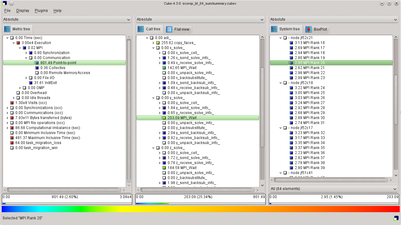
Examination of the summary result (see Figure SummaryExperiment for a screenshot and Section Using the Cube browser for a brief summary of how to use the Cube browser) shows that 97% of the overall CPU allocation time is spent executing computational user functions, while 2.6% of the time is spent in MPI point-to-point communication functions and the remainder scattered across other activities. The point-to-point time is almost entirely spent in MPI_Wait calls inside the three solver functions x_solve, y_solve and z_solve, as well as an MPI_Waitall in the boundary exchange routine copy_faces. Execution time is also mostly spent in the solver routines and the boundary exchange, however, inside the different solve_cell, backsubstitute and compute_rhs functions. While the aggregated time spent in the computational routines seems to be relatively balanced across the different MPI ranks (determined using the box plot view in the right pane), there is quite some variation for the MPI_Wait / MPI_Waitall calls.

"SummaryExperiment": Screenshot of a summary experiment result in the Cube report browser.

Using the Cube browser

The following paragraphs provide a very brief introduction to the usage of the Cube analysis report browser. To make effective use of the GUI, however, please also consult the Cube User Guide [3].

Cube is a generic user interface for presenting and browsing performance and debugging information from parallel applications. The underlying data model is independent from particular performance properties to be displayed. The Cube main window (see Figure SummaryExperiment) consists of three panels containing tree displays or alternate graphical views of analysis reports. The left panel shows performance properties of the execution, such as time or the number of visits. The middle pane shows the call tree or a flat profile of the application. The right pane either shows the system hierarchy consisting of, e.g., machines, compute nodes, processes, and threads, a topological view of the application's processes and threads (if available), or a box plot view showing the statistical distribution of values across the system. All tree nodes are labeled with a metric value and a color-coded box which can help in identifying hotspots. The metric value color is determined from the proportion of the total (root) value or some other specified reference value, using the color scale at the bottom of the window.

A click on a performance property or a call path selects the corresponding node. This has the effect that the metric value held by this node (such as execution time) will be further broken down into its constituents in the panels right of the selected node. For example, after selecting a performance property, the middle panel shows its distribution across the call tree. After selecting a call path (i.e., a node in the call tree), the system tree shows the distribution of the performance property in that call path across the system locations. A click on the icon to the left of a node in each tree expands or collapses that node. By expanding or collapsing nodes in each of the three trees, the analysis results can be viewed on different levels of granularity (inclusive vs. exclusive values).

All tree displays support a context menu, which is accessible using the right mouse button and provides further options. For example, to obtain the exact definition of a performance property, select "Online Description" in the context menu associated with each performance property. A brief description can also be obtained from the menu option "Info".