 |
Cube GUI User Guide
(CubeGUI 4.6, revision ff50a50d)
Introduction in Cube GUI and its usage
|
|
Cube GUI User Guide
(CubeGUI 4.6, revision ff50a50d)
Introduction in Cube GUI and its usage
|
This section explains how to use the CUBE-QT display component. After installation, the executable "cube" can be found in the specified directory of executables (specifiable by the ``prefix'' argument of configure, see the CUBE Installation Manual). The program supports as an optional command-line argument the name of a cube file that will be opened upon program start.
After a brief description of the basic principles, different components of the GUI will be described in detail.
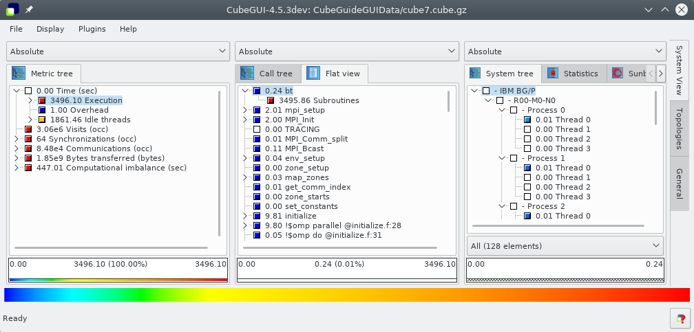
The CUBE-QT display has three tree browsers, each of them representing a dimension of the performance space (figure gui). Per default, the left tree displays the metric dimension, the middle tree displays the program dimension, and the right tree displays the system dimension. The nodes in the metric tree represent metrics. The nodes in the program dimension can have different semantics depending on the particular view that has been selected. In Figuregui, they represent call paths forming a call-tree. The nodes in the system dimension represent machines, nodes, processes, or threads from top to bottom.
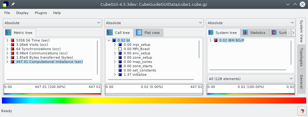
Each node is associated with a value, which is called the severity and is displayed simultaneously using a numerical value as well as a colored square. Colors enable the easy identification of nodes of interest even in a large tree, whereas the numerical values enable the precise comparison of individual values. The sign of a value is visually distinguished by the relief of the colored square. A raised relief indicates a positive sign, a sunken relief indicates a negative sign.
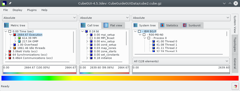
Users can perform two basic types of actions: selecting a node or expanding/collapsing a node. In the metric-tree in figure gui, the metric Execution is selected. Selecting a node in a tree causes the other trees on its right to display values for that selection. For the example of figure gui, the metric-tree displays the total metric values over all call-tree and system nodes, the call-tree displays values for the Execution metric over all system entities, and the system-tree for the Execution metric and the adi call-tree node. Briefly, a tree is always an aggregation over all selected nodes of its neighboring trees to the left.
Collapsed nodes with a subtree that is not shown are marked by a [+] sign, expanded nodes with a visible subtree by a [-] sign. You can expand/collapse a node by left-clicking on the corresponding [+]/[-] signs. Collapsed nodes have inclusive values, i.e., their severity is the sum of the severities over the whole collapsed subtree. For the example of Figuregui, the Execution metric value  is the total time for all executions. On the other hand, the displayed values of expanded nodes are their exclusive values. E.g., the expanded
 Execution metric node in Figure gui2 shows that the program needed  seconds for execution other than
 MPI.
Note that expanding/collapsing a selected node causes the change of the current values in the trees on its right-hand side. As explained above, in our example in Figure gui the call-tree displays values for the Execution metric over all system entities. Since the Execution node is collapsed, the call-tree severities are computed for the whole Execution metric's subtree. When expanding the selected Execution node, as shown in Figure gui2, the call-tree displays values for the Execution metric without the MPI metric.
The GUI consists (from top to bottom) of
Subsections:
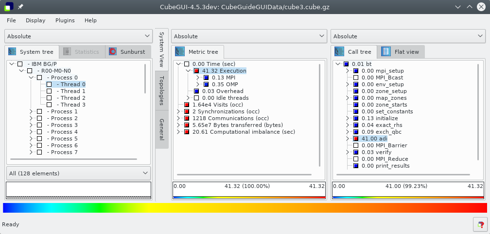
The three resizable panes offer different views: the metric, the call, and the system pane. You can switch between the different tabs of a pane by left-clicking on the desired tab at the top of the pane. Note that the order of the panes can be changed (see the description of the menu item Display => Dimension order in Section Menu Bar ).
The metric pane provides only the metric-tree browser. The call pane offers a call-tree browser and a flat call profile. If OpenMP tasks have been instrumented, an additional task-tree is inserted. The system pane has a system-tree browser. Tree browsers also provide a context menu.
The menu bar consists of four menus: a file menu, a display menu, a plugin menu and a help menu. Some menu functions also have a keyboard shortcut, which is written besides the menu item's name in the menu. E.g., you can open a file with Ctrl+O without going into the menu. A short description of the menu items is visible in the status bar if you stay for a short while with the mouse above a menu item.
File: The file menu offers the following functions:
Open (Ctrl+O): Offers a selection dialog to open a CUBE file. In case of an already opened file, it will be closed before a new file gets opened. If a file got opened successfully, it gets added to the top of the recent files list (see below). If it was already in the list, it is moved to the top.
Open URL: Opens a remote file dialog (see section Client-Server)
Save as (Ctrl+S): Offers a selection dialog to save a copy of a CUBE file. Opened CUBE file stays loaded in cube.
Close (Ctrl+W): Closes the currently opened CUBE file. Disabled if no file is opened.
Open external: Opens a file for the external percentage value mode (see section Value modes).
Close external: Closes the current external file and removes all corresponding data. Disabled if no external file is opened.
Settings: Offers saving, loading, and deletion of global settings. Global settings don't depend on the loaded cube file and are saved in a system specific format. These settings e.g. store the appearance of the application like the widget sizes, color and precision settings, the order of panes, etc.
"Restore last state" depends on a loaded cube file. If it is activated, the state of the cube file, e.g. selected and expanded items, is saved before the cube file is closed and restored after loading.
Screenshot: The function offers you to save a screen snapshot in a PNG file. Unfortunately the outer frame of the main window is not saved, only the application itself.
Quit (Ctrl+Q): Closes the application.
 opened files are offered for re-opening, the top-most being the most recently opened one. A full path to the file is visible in the status bar if you move the mouse above one of the recent file items in the menu.
 Display: The display menu offers the following functions:
Dimension order: As explained above, CUBE has three resizable panes. Initially the metric pane is on the left, the call pane is in the middle, and the system pane is on the right-hand side. However, sometimes you may be interested in other orders, and that is what this menu item is about. It offers all possible pane orderings. For example, assume you would like to see the metric and call values for a certain thread. In this case, you could place the system pane on the left, the metric pane in the middle, and the call pane on the right, as shown in Figure order. Note that in panes to the left of the metric pane no meaningful valuescan be presented, since they miss a reference metric; in this case values are specified to be undefined, denoted by a ``-'' (minus) sign.
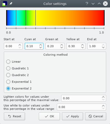
Choose/Edit colormap: Allows for selection of color maps and changing of color settings in a new dialog. In the configuration dialog, the Ok button applies the settings to the display and closes the dialog, the Apply button applies the settings to the display, and Cancel cancels all changes since the dialog was opened (even if "Apply" was pressed in between) and closes the dialog.
The configuration dialog in Figure coloring shows the default color map for Cube. Other colormaps may be added using plugins, see for example the Advanced Colormap Plugin (Advanced Color Map Plugin). At the top of the dialog you see a color legend with some vertical black lines, showing the position of the color scale start, the colors cyan, green, and yellow, and the color scale end. These lines can be dragged with the left mouse button, or their position can also be changed by typing in some values between  (left end) and
  (right end) below the color legend in the corresponding spins.
The different coloring methods offer different functions to interpolate the colors at positions between the data points specified above.
With the upper spin below the coloring methods you can define a threshold percentage value between and  , below which colors are lightened. The nearer to the left end of the color scale, the stronger the lightening (with linear increase).
With the spin at the bottom of the dialog you can define a threshold percentage value between and , below which values should be colored white.
Customize style sheets Opens a dialog to define Customization with Qt Stylesheets to change e.g. the fonts and sizes of GUI elements.
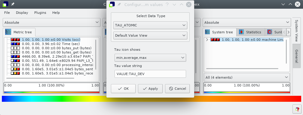
Configure value view: This menu item opens a dialog in which the icon and the textual value representation of the tree items can be configured. Depending on the data type of the selected metric, additional options and additional value view plugins may be available. For metrics that consist of more than one value, e.g. tau metrics (see figure tau-value-view), the user can select which value should be used for the icon and which values for the following text.
Precision: Activating this menu item opens a dialog for precision settings (see Figure precision). Besides Ok and Cancel, the dialog offers an Apply button, that applies the current dialog settings to the display. Pressing Cancel undoes all changes due to the dialog, even if you already pressed Apply previously, and closes the dialog. Ok applies the settings and closes the dialog.
It consists of two parts: precision settings for the tree displays, and precision settings for the selected value info widgets and the topology displays. For both formats, three values can be defined:
 with x: Here you can define above which threshold scientific notation should be used. E.g., the value 1000 is displayed as 1000 if this value is larger then 3 and as
  otherwise.
  with x: Due to inexact floating point representation, it often happens that users wish to round down values very near by zero to zero. Here you can define the threshold below which this rounding should take place. E.g., the value 0.0001 is displayed as 0.0001 if this value is larger than 3 and as zero otherwise.
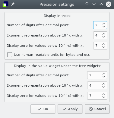
Trees: This menu offers options to change the contents and the appearance of the items of all trees.
Font and colors: Opens a dialog to define Customization with Qt Stylesheets to change e.g. the fonts and sizes of GUI elements.
Configure Tree Item Marker In this dialog, you can change the appearance of defined tree item markers. You may choose if the items should be marked with a special background color or with an icon (see Tree Item Marker).
Demangle Function Names (only call trees) If this option is enabled (default), cube tries to demangle function names.
Shorten Function Names (only call trees) This menu item opens a dialog in which you can hide parts of long function names. You may hide argument lists and return values of C++ functions. You may also hide namespaces, class and templates from C++ function names. For Fortran subroutines, module names can be hidden.
Enable presentation mode If the presentation mode is enable, a mouse icon is shown next to the cursor
Plugins: The plugin menu allows the user to define which plugins are laoded. For each loaded plugin, a submenu is added. The submenu contains a menu item to enable or disable the plugin and the plugin may add additional menu items.
Getting started: Opens a dialog with some basic information on the usage of CUBE.
Mouse and keyboard control: Lists mouse and keyboard controls as given in Section Source Code Viewer Keyboard control.
What's this?: Here you can get more specific information on parts of the CUBE GUI. If you activate this menu item, you switch to the ``What's this?'' mode. If you now click on a widget, an appropriate help text is shown. The mode is left when help is given or when you press Esc.
Another way to ask the question is to move the focus to the relevant widget and press Shift+F1.
About: Opens a dialog with release information.
Plugin documentation shows the plugin documentation in a browser window
Selected metric description: Opens a new window showing the description of the currently selected metric, equivalent to Documentation in the metric-tree context menu. Disabled if online documentation is unavailable.
Selected region description: Opens a new window showing the description of the currently selected region, equivalent to Documentation in the call-tree context menu. Disabled if online documentation is unavailable.
Each tree view has its own value mode combobox, a drop-down menu above the tree, where it is possible to change the way the severity values are displayed.
The default value mode is the Absolute value mode. In this mode, as explained below, the severity values from the CUBE file are displayed. However, sometimes these values may be hard to interpret, and in such cases other value modes can be applied. Basically, there are three categories of additional value modes.
The first category presents all severities in the tree as percentage of a reference value. The reference value can be the absolute value of a selected or a root node from the same tree or in one of the trees on the left-hand side. For example, in the Own root percent value mode the severity values are presented as percentage of the own root's (inclusive) severity value. This way you can see how the severities are distributed within the tree. All the value modes (Own root percent – System selection percent) fall into this category.
All nodes of trees on the left-hand side of the metric-tree have undefined values. (Basically, we could compute values for them, but it would sum up the severities over all metrics, that have different meanings and usually even different units, and thus those values would not have much expressiveness.) Since we cannot compute percentage values based on undefined reference values, such value modes are not supported. For example, if the call-tree is on the left-hand side, and the metric-tree is in the middle, then the metric-tree does not offer the Call root percent mode.
Depending on the type and position of the tree, the following value modes may be available:
Note that in all modes, only the leaf nodes in the system hierarchy (i.e., processes or threads) have associated severity values. All other hierarchy levels (i.e., machines, nodes and eventually processes) are only used to structure the hierarchy. This means that their severity is undefined—denoted by a ``-'' (minus) sign—when they are expanded.
By default, all system resources (typically threads) are included when determining boxplot statistics. Other defined subsets can be chosen from the combobox below the boxplot, such as ``Visited'' threads which are only those threads that visited the currently selected callpath. The current subset is retained until another is explicitly chosen or a new subset is defined.
Additional subsets are defined from the system-tree with the Define subset context menu using the currently selected threads via multiple selection (Ctrl+<left-mouse click>) or with the Find Items context menu selection option.
A tree browser displays different hierarchical data structures in form of trees. Currently supported tree types are metric-trees, call-trees and their flat call profiles, and system-trees. The structure of the displayed data is common in all trees: The indentation of the tree nodes reflects the hierarchical structure. Expandable nodes, i.e., nodes with non-hidden children, are equipped with a [+]/[-] sign ([+] for collapsed and [-] for expanded nodes). Furthermore, all nodes have a color icon, a value, and a label.
The value of a node is computed, as explained earlier, basing on the current selections in the trees on the left-hand side and on the current value mode. The precision of the value display in trees can be modified, see the menu item Display => Precision in Section Menu Bar. The color icon reflects the position of the node's value between and a maximal value. These maximal value is the maximal value in the tree for the absolute value mode, or otherwise. See the menu item Display => Choose colormap in Section Menu Bar and the context menu item Min/max values in the context menu description below for color settings.
A label in the metric-tree shows the metric's name. A label in the call-tree shows the last callee of a particular call path. If you want to know the complete call path, you must read all labels from the root down to the particular node you are interested in. After switching to the flat profile view (see below), labels in the flat call profile denote methods or program regions. A label in the system-tree shows the name of the system resource it represents, such as a node name or a machine name. Processes and threads are usually identified by a rank number, but it is possible to give them specific names when creating a CUBE file. The thread level of single-threaded applications is hidden. Multiple root nodes are supported.
After opening a data set, the middle panel shows the call-tree of the program. However, a user might wish to know which fraction of a metric can be attributed to a particular region (e.g., method) regardless of from where it was called. In this case, you can switch from the call-tree view (default) to the flat-profile view (Figure region). In the flat-profile view, the call-tree hierarchy is replaced with a source-code hierarchy consisting of two levels: regions and their subroutines. Any subroutines are displayed as a single child node labeled Subroutines. A subroutine node represents all regions directly called from the region above. In this way, you are able to see which fraction of a metric is associated with a region exclusively, that is, without its regions called from there.
Tree displays are controlled by the left and right mouse buttons and some keyboard keys. The left mouse button is used to select or expand/collapse a node: You can expand/collapse a node by left-clicking on the attached [+]/[-] sign, and select it by left-clicking elsewhere in the node's line. To select multiple items, Ctrl+<left-mouse click> can be used. Selection without the Ctrl key deselects all previously selected nodes and selects the clicked node. In single-selection mode you can also use the up/down arrows to move the selection one node up/down. The right mouse button is used to pop up a context menu with node-specific information, such as online documentation (see the description of the context menu below).
Each tree has its own context menu which can be activated by a right mouse click within the tree's window. If you right-click on one of the tree's nodes, this node gets framed, and serves as a reference node for some of the menu items. If you click outside of tree items, there is no refernce node, and some menu items are disabled.
The context menu consists, depending on the type of the tree, of some of the following items. If you move the mouse over a context menu item, the status bar displays some explanation of the functionality of that item.
Collapse all: Collapses all nodes in the tree.
Collapse subtree: Enabled only if there is a reference node. It collapses all nodes in the subtree of the reference node (including the reference node).
Expand current level: For system-trees only. Shows all nodes that are on the same hierarchy level as the chosen one by expanding their parents.
Dynamic hiding: Not available for metric-trees. This menu item activates dynamic hiding. All currently hidden nodes get shown. You are asked to define a percentage threshold between and . All nodes whose color position on the color scale (in percent) is below this threshold get hidden. As default value, the color percentage position of the reference node is suggested, if you right-clicked over a node. If not, the default value is the last threshold. The hiding is called dynamic, because upon value changes (caused for example by changing the node selection) hiding is re-computed for the new values. In other words, value changes may change the visibility of the nodes.
During dynamic hiding, for expanded nodes with some hidden children and for nodes with all of its children hidden, their displayed (exclusive) value includes the hidden children's inclusive value. The percentage of the hidden children is shown in brackets next to this aggregate value.
Static hiding: Not available for metric-trees. This menu item activates static hiding. All currently hidden nodes stay hidden. Additionally, you can hide and show nodes using the now enabled sub-items:
Like for dynamic hiding, for expanded nodes with some hidden children and for nodes with all of its children hidden, their displayed (exclusive) value includes the hidden children's inclusive value. The percentage of the hidden children is shown in brackets next to this aggregate value.
No hiding: Not available for metric-trees. This menu item deactivates any hiding, and shows all hidden nodes.
Find items: For all trees. Opens a text input widget below the corresponding tree to enter a regular expression to search for. If the user called the context menu over an item, the default text is the name of the reference node. All non-hidden nodes whose names contain the given expression are marked with a yellow background, and all collapsed nodes whose subtree contains such a non-hidden node by a light yellow background.
The button expand all expands all found items.
The button select all selects all found items. The selected items may still be collapsed.
The arrow buttons select the next or the previous found item. The shortcuts for these actions are F3 and Shift+F3.
Clear found items: For all trees. Removes the background markings of the preceding "find items" action.
Define subset: Only for system-tree. Uses the currently selected system resources (e.g., from a preceding Find items) to create a new subset of all system resources (typically threads) with the provided name. This is added to the combobox at the bottom of the system-tree and boxplot statistics panes, and becomes the currently active subset for which statistics are calculated.
Info/Documentation: For metric and call-trees Shows combined information about the selected metric an call-tree items in a new tab. For the selected metric, information about display, unique name, data type, unit of measurements and kind of metric is shown. If the metric is derived, the CubePL expression is shown.
For the selected call path, information about call path id (to use it with command line tools like cube_dump), region begining line, region ending line, region module, url with the online help and finally description of the region is shown.
If online documentation for the reference node is available, it is shown in a html widget below the informataion panels. For example, metrics might point to an online documentation explaining their semantics, or regions representing library functions might point to the corresponding library documentation.
Disabled, if not clicked over metric or call path item.
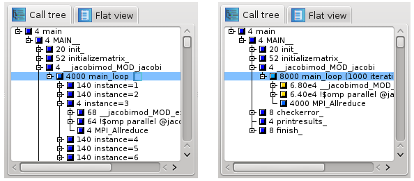
Hide iterations: Only visible for calltree items that are recognized or manually defined as loop (see "Set as loop" below). By activating, all children of the loop are hidden. The grandchildren are shown and its values for the different iterations are aggregated (see Figurelooplabel).
Call site: For call-trees only. Enabled only if there is a reference node. Offers information about the caller of the reference node.
Called region: For call-trees only. Enabled only if there is a reference node. Offers information about the reference node.
Min/max values: Not for metric-trees. Here you can activate and deactivate the application of user-defined minimal and maximal values for the color extremes, i.e., the values corresponding to the left and right end of the color legend. If you activate user-defined values for the color extremes, you are asked to define two values that should correspond to the minimal and to the maximal colors. All values outside of this interval will get the color gray. Note that canceling any of the input windows causes no changes in the coloring method. If user-defined min/max values are activated, the selected value information widget (see Section Selected value info) displays a (u)'' foruser-defined'' behind the minimal and maximal color values.
Statistics: Only available if a statistics file for the current CUBE file is provided. Displays statistical information about the instances of the selected metric in the form of a box plot. For an in-depth explanation of this feature see subsection Statistical information about performance patterns.
Max severity in trace browser: Only available for metric and call-trees and only if a statistics file providing information about the most severe instance(s) of the selected metric is present. If CUBE is already connected to a trace browser (via File => Connect to trace browser), the timeline display of the trace browser is zoomed to the position of the occurrence of the most severe pattern so that the cause for the pattern can be examined further. For a more detailed explanation of this feature see subsection Display of most severe pattern instances using a trace browser.
Cut call tree/Cut selected call tree items This context menu is enabled, if the right mouse button is pressed on a call tree item. If the mouse button is pressed and the item below the mouse pointer is part of a group of selected items, the action affects all selected items. Otherwise, only the item below the mouse item will be modified. The menu offers different modification possibilities:
Sort by order of definition: Restores the original order.
Below each pane there is a selected value information widget. If no data is loaded, the widget is empty. Otherwise, the widget displays more extensive and precise information about the selected values in the tree above. This information widget and the topologies may have different precision settings than the trees, such that there is the possibility to display more precise information here than in the trees (see Section Menu Bar, menu Display => Precision).
The widget has a 3-line display. The first line displays at most 4 numbers. The left-most number shows the smallest value in the tree (or in any percentage value mode for trees, or the user-defined minimal value for coloring if activated), and the right-most number shows the largest value in the tree (or in any percentage value mode in trees, or the user-defined maximal value for coloring if activated). Between these two numbers the current value of the selected node is displayed, if it is defined. Additionally, in the absolute value mode it is followed by the percentage of the selected value on the scale between the minimal and maximal values, shown in brackets. Note that the values of expanded non-leaf system nodes and of nodes of trees on the left-hand side of the metric-tree are not defined. If the value mode is not the absolute value mode, then in the second line similar information is displayed for the absolute values in a light gray color.
In case of multiple selection, the information refers to the sum of all selected values. In case of multiple selection in system trees in the peer distribution and in the peer percent modes, this sum does not state any valuable information, but is displayed for consistency reasons.
If the widget width is not large enough to display all numbers in the given precision, then a part of the number displays get cut down and a ``  '' indicates that not all digits could be displayed.
Below these numbers, in the third line, a small color bar shows the position of the color of the selected node in the color legend. In case of undefined values, the legend is filled with a gray grid.
By default, the colors are taken from a spectrum ranging from blue over cyan, green, and yellow to red, representing the whole range of possible values. You can change the color settings in the menu,Display => Choose colormap, see Section Menu Bar. Exact zero values are represented by the color white (in topologies you can decide whether you would like to use white or the minimal color, see Section System Topology Plugin, menu Topology).
The status bar displays some status information, like state of execution for longer procedures, hints for menus the mouse pointing at etc.
The status bar shows the most recent log message. By clicking on it, the complete log becomes visible.
 |
Copyright © 1998–2021 Forschungszentrum Jülich GmbH,
Jülich Supercomputing Centre
Copyright © 2009–2015 German Research School for Simulation Sciences GmbH, Laboratory for Parallel Programming |