 |
Scalasca
(Scalasca 2.6.2, revision 30af1b6e)
Scalable Performance Analysis of Large-Scale Applications
|
|
Scalasca
(Scalasca 2.6.2, revision 30af1b6e)
Scalable Performance Analysis of Large-Scale Applications
|
While summary profiles only provide process- or thread-local data aggregated over time, event traces contain detailed time-stamped event data which also allows to reconstruct the dynamic behavior of an application. This enables tools such as the Scalasca trace analyzer to provide even more insights into the performance behavior of an application, for example, whether the time spent in MPI communication is real message processing time or incurs significant wait states (i.e., intervals where a process sits idle without doing useful work waiting for data from other processes to arrive).
Trace collection and subsequent automatic analysis by the Scalasca trace analyzer can be enabled using the -t option of scalasca -analyze. Since this option enables trace collection in addition to collecting a summary measurement, it is often used in conjunction with the -q option which turns off measurement entirely. (Note that the order in which these two options are specified matters: First turn off measurement using -q, then enable tracing with -t.)
SCOREP_TOTAL_MEMORY setting)! Otherwise, you may easily fill up your disks and suffer from uncoordinated intermediate trace buffer flushes, which typically render such traces to be of little (or no) value!For our example measurement, scoring of the initial summary report in Section Optimizing the measurement configuration with the filter applied estimated a total memory requirement of 30 MiB per process (which could be verified by re-scoring the filtered summary measurement). As this exceeds the default SCOREP_TOTAL_MEMORY setting of 16 MiB, use of the prepared filtering file alone is not yet sufficient to avoid intermediate trace buffer flushes. In addition, the SCOREP_TOTAL_MEMORY setting has to be adjusted accordingly before starting the trace collection and analysis. For the example measurement shown below, a slightly larger memory buffer of 32 MiB is used, although this is not strictly necessary. As an alternative, the filtering file could be extended to also exclude additional routines from measurement (e.g., binvrhs) to further reduce the trace buffer requirements at the expense of loosing details.
With this setting in place, a trace measurement can now be collected and subsequently analyzed by the Scalasca trace analyzer. Note that renaming or removing the summary experiment directory is not necessary, as trace experiments are created with suffix "trace".
  $ export SCOREP_TOTAL_MEMORY=32M
  $ scalasca -analyze -q -t -f npb-bt.filt mpiexec -n 144 ./bt.D.144
  S=C=A=N: Scalasca 2.5 trace collection and analysis
  S=C=A=N: ./scorep_bt_144_trace experiment archive
  S=C=A=N: Mon Mar 18 13:57:08 2019: Collect start
  mpiexec -n 144 ./bt.D.144


   NAS Parallel Benchmarks 3.3 -- BT Benchmark

   No input file inputbt.data. Using compiled defaults
   Size:  408x 408x 408
   Iterations:  250    dt:   0.0000200
   Number of active processes:   144

   Time step    1
   Time step   20
   Time step   40
   Time step   60
   Time step   80
   Time step  100
   Time step  120
   Time step  140
   Time step  160
   Time step  180
   Time step  200
   Time step  220
   Time step  240
   Time step  250
   Verification being performed for class D
   accuracy setting for epsilon =  0.1000000000000E-07
   Comparison of RMS-norms of residual
             1 0.2533188551738E+05 0.2533188551738E+05 0.1499315900507E-12
             2 0.2346393716980E+04 0.2346393716980E+04 0.8546885387975E-13
             3 0.6294554366904E+04 0.6294554366904E+04 0.2745293523008E-14
             4 0.5352565376030E+04 0.5352565376030E+04 0.8376934357159E-13
             5 0.3905864038618E+05 0.3905864038618E+05 0.6650300273080E-13
   Comparison of RMS-norms of solution error
             1 0.3100009377557E+03 0.3100009377557E+03 0.1373406191445E-12
             2 0.2424086324913E+02 0.2424086324913E+02 0.1600422929406E-12
             3 0.7782212022645E+02 0.7782212022645E+02 0.4090394153928E-13
             4 0.6835623860116E+02 0.6835623860116E+02 0.3596566920650E-13
             5 0.6065737200368E+03 0.6065737200368E+03 0.2605201960010E-13
   Verification Successful


   BT Benchmark Completed.
   Class           =                        D
   Size            =            408x 408x 408
   Iterations      =                      250
   Time in seconds =                   227.78
   Total processes =                      144
   Compiled procs  =                      144
   Mop/s total     =                256110.17
   Mop/s/process   =                  1778.54
   Operation type  =           floating point
   Verification    =               SUCCESSFUL
   Version         =                    3.3.1
   Compile date    =              18 Mar 2019

   Compile options:
      MPIF77       = scorep mpifort
      FLINK        = $(MPIF77)
      FMPI_LIB     = (none)
      FMPI_INC     = (none)
      FFLAGS       = -O2
      FLINKFLAGS   = -O2
      RAND         = (none)


   Please send feedbacks and/or the results of this run to:

   NPB Development Team
   Internet: npb@nas.nasa.gov


  S=C=A=N: Mon Mar 18 14:01:04 2019: Collect done (status=0) 236s
  S=C=A=N: Mon Mar 18 14:01:04 2019: Analyze start
  mpiexec -n 144 scout.mpi ./scorep_bt_144_trace/traces.otf2
  SCOUT   (Scalasca 2.5)
  Copyright (c) 1998-2019 Forschungszentrum Juelich GmbH
  Copyright (c) 2009-2014 German Research School for Simulation Sciences GmbH

  Analyzing experiment archive ./scorep_bt_144_trace/traces.otf2

  Opening experiment archive ... done (0.008s).
  Reading definition data    ... done (0.017s).
  Reading event trace data   ... done (0.280s).
  Preprocessing              ... done (0.366s).
  Analyzing trace data       ... done (2.511s).
  Writing analysis report    ... done (0.104s).

  Max. memory usage         : 170.812MB
  *** WARNING ***
  40472 clock condition violations detected:
     Point-to-point:    40472
     Collective    :        0
  This usually leads to inconsistent analysis results.

  Try running the analyzer using the '--time-correct' command-line
  option to apply a correction algorithm.


  Total processing time     : 3.383s
  S=C=A=N: Mon Mar 18 14:01:09 2019: Analyze done (status=0) 5s
  Warning: 3.686GB of analyzed trace data retained in ./scorep_bt_144_trace/traces!
  S=C=A=N: ./scorep_bt_144_trace complete.

  $ ls scorep_bt_144_trace
  MANIFEST.md  scorep.filter  scout.cubex  trace.cubex  traces.def   trace.stat
  scorep.cfg   scorep.log     scout.log    traces       traces.otf2
As can be seen, the scalasca -analyze convenience command automatically initiates the trace analysis after successful trace collection. Besides the already known files MANIFEST.md, scorep.cfg, scorep.filter, and scorep.log, the generated experiment directory scorep_bt_144_trace now contains artifacts related to trace measurement and analysis:
traces.otf2, the global definitions file traces.def, and the per-process data in the traces/ directory,scout.log, and finallyscout.cubex and trace.stat.The Scalasca trace analyzer also warned about a number of point-to-point clock condition violations it detected. A clock condition violation is a violation of the logical event order that can occur when the local clocks of the individual compute nodes are insufficiently synchronized. For example, based on the measured timestamps, a receive operation may appear to have finished before the corresponding send operation started—something that is obviously not possible. The Scalasca trace analyzer includes a correction algorithm [2] that can be applied in such cases to restore the logical event order, while trying to preserve the length of intervals between local events in the vicinity of the violation.
To enable this correction algorithm, the --time-correct command-line option has to be passed to the Scalasca trace analyzer. However, since the analyzer is implicitly started through the scalasca -analyze command, this option has to be set using the SCAN_ANALYZE_OPTS environment variable, which holds command-line options that scalasca -analyze should forward to the trace analyzer. Instead of collecting and analyzing a new experiment, an existing trace measurement can also be re-analyzed using the -a option of the scalasca -analyze command:
  $ export SCAN_ANALYZE_OPTS="--time-correct"
  $ scalasca -analyze -a mpiexec -n 144 ./bt.D.144
  S=C=A=N: Scalasca 2.5 trace analysis
  S=C=A=N: ./scorep_bt_144_trace experiment archive
  S=C=A=N: Mon Mar 18 14:02:57 2019: Analyze start
  mpiexec -n 144 scout.mpi --time-correct ./scorep_bt_144_trace/traces.otf2
  SCOUT   (Scalasca 2.5)
  Copyright (c) 1998-2019 Forschungszentrum Juelich GmbH
  Copyright (c) 2009-2014 German Research School for Simulation Sciences GmbH

  Analyzing experiment archive ./scorep_bt_144_trace/traces.otf2

  Opening experiment archive ... done (0.013s).
  Reading definition data    ... done (0.023s).
  Reading event trace data   ... done (0.615s).
  Preprocessing              ... done (0.478s).
  Timestamp correction       ... done (0.463s).
  Analyzing trace data       ... done (2.653s).
  Writing analysis report    ... done (0.106s).

  Max. memory usage         : 174.000MB

  	# passes        : 1
  	# violated      : 9450
  	# corrected     : 23578735
  	# reversed-p2p  : 9450
  	# reversed-coll : 0
  	# reversed-omp  : 0
  	# events        : 301330922
  	max. error      : 0.000048 [s]
  	error at final. : 0.000000 [%]
  	Max slope       : 0.394363334

  Total processing time     : 4.448s
  S=C=A=N: Mon Mar 18 14:03:07 2019: Analyze done (status=0) 10s
  Warning: 3.686GB of analyzed trace data retained in ./scorep_bt_144_trace/traces!
  S=C=A=N: ./scorep_bt_144_trace complete.
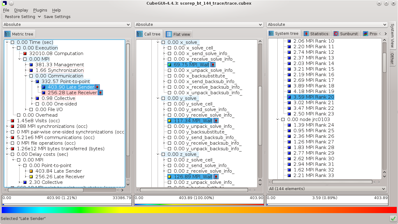
Similar to the summary report, the trace analysis report can finally be post-processed and interactively explored using the Cube report browser, again using the scalasca -examine convenience command:
  $ scalasca -examine scorep_bt_144_trace
  INFO: Post-processing trace analysis report (scout.cubex)...
  INFO: Displaying ./scorep_bt_144_trace/trace.cubex...
The report generated by the Scalasca trace analyzer is again a profile in CUBE4 format, however, enriched with additional performance properties. Examination shows that about two-thirds of the time spent in MPI point-to-point communication is waiting time, split into roughly 60% in Late Sender and 40% in Late Receiver wait states (see Figure TraceAnalysis). While the execution time in the solve_cell routines looked relatively balanced in the summary profile, examination of the Critical path imbalance metric shows that these routines in fact exhibit a small amount of imbalance, which is likely to cause the wait states at the next synchronization point. This can be verified using the Late Sender delay costs metric, which confirms that the solve_cells as well as the y_backsubstitute and z_backsubstitute routines are responsible for almost all of the Late Sender wait states. Likewise, the Late Receiver delay costs metric shows that the majority of the Late Receiver wait states are caused by the solve_cells routines as well as the MPI_Wait calls in the solver routines, where the latter indicates a communication imbalance or an inefficient communication pattern.
 |
Copyright © 1998–2025 Forschungszentrum Jülich GmbH,
Jülich Supercomputing Centre
Copyright © 2009–2015 German Research School for Simulation Sciences GmbH, Laboratory for Parallel Programming |