Abstract

CUBE is a presentation component suitable for displaying performance data for parallel programs including MPI and OpenOpenMP applications. Program performance is represented in a multi-dimensional space including various program and system resources. The tool allows the interactive exploration of this space in a scalable fashion and browsing the different kinds of performance behavior with ease. CUBE also includes a library to read and write performance data as well as operators to compare, integrate, and summarize data from different experiments. This user manual provides instructions of how to use the CUBE display, how to use the operators, and how to write CUBE files.

The version 4 of CUBE implementation has an incompatible API and file format to preceding versions.

Introduction

CUBE (CUBE Uniform Behavioral Encoding) is a presentation component suitable for displaying a wide variety of performance data for parallel programs including MPI and OpenOpenMP applications. CUBE allows interactive exploration of the performance data in a scalable fashion.cube_ Scalability is achieved in two ways: hierarchical decomposition of individual dimensions and aggregation across different dimensions. All metrics are uniformly accommodated in the same display and thus provide the ability to easily compare the effects of different kinds of program behavior.

CUBE has been designed around a high-level data model of program behavior called the cube performance space. The CUBE performance space consists of three dimensions: a metric dimension, a program dimension, and a system dimension. The metric dimension contains a set of metrics, such as communication time or cache misses. The program dimension contains the program's call tree, which includes all the call paths onto which metric values can be mapped. The system dimension contains the items executing in parallel, which can be processes or threads depending on the parallel programming model. Each point $ (m, c, s) $ of the space can be mapped onto a number representing the actual measurement for metric $ m $ while the control flow of process/thread $ s $ was executing call path $ c $ . This mapping is called the severity of the performance space.

Each dimension of the performance space is organized in a hierarchy. First, the metric dimension is organized in an inclusion hierarchy where a metric at a lower level is a subset of its parent. For example, communication time is a subset of execution time. Second, the program dimension is organized in a call-tree hierarchy. However, sometimes it can be advantageous to abstract away from the hierarchy of the call tree, for example if one is interested in the severities of certain methods, independently of the position of their invocations. For this purpose CUBE supports also flat call profiles, that are represented as a flat sequence of all methods. Finally, the system dimension is organized in a multi-level hierarchy consisting of the levels: machine, node, process, and thread.

CUBE also provides a library to read and write instances of the previously described data model in the form of a file (which is a file anchor.xml inside of the envelope. The data part contains the actual severity numbers to be mapped onto the different elements of the performance space and stored in binary format in various files inside of the envelope.

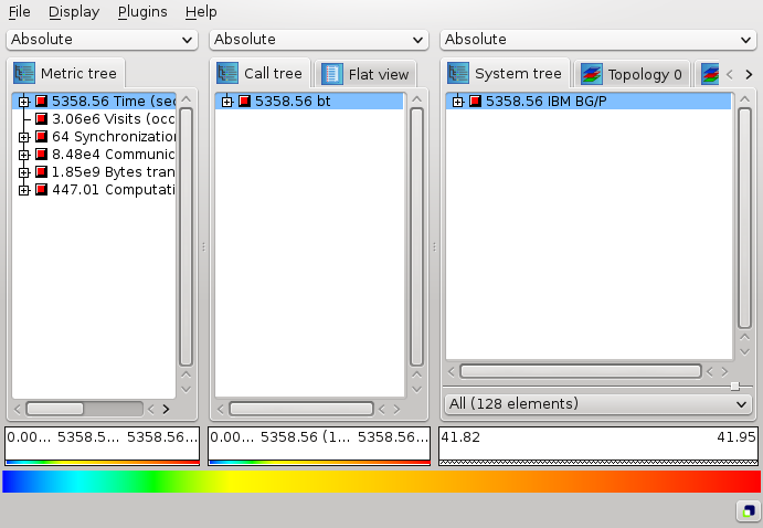
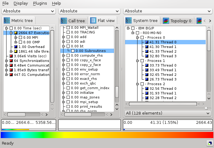
The display component can load such a file and display the different dimensions of the performance space using three coupled tree browsers (figure ). The browsers are connected in such a way that you can view one dimension with respect to another dimension. The connection is based on selections: in each tree you can select one or more nodes. For example, in Figure the Execution metric, the adi call path node, and Process 0 are selected. For each tree, the selections in the trees on its left-hand-side (if any) restrict the considered data: The metric nodes aggregate data over all call path nodes and all system items, the call tree aggregates data for the Execution metric over all system nodes, and each node of the system tree shows the severity for the Execution metric of the adi call path node for this system node.

If the CUBE file contains topological information, the distribution of the performance metric across the topology can be examined using the topology view. Furthermore, the display is augmented with a source-code display that shows the position of a call site in the source code.

As performance tuning of parallel applications usually involves multiple experiments to compare the effects of certain optimization strategies, CUBE includes a feature designed to simplify cross-experiment analysis. The CUBE algebra is an extension of the framework for multi-execution performance tuning by Karavanic and Miller and offers a set of operators that can be used to compare, integrate, and summarize multiple CUBE data sets. The algebra allows the combination of multiple CUBE data sets into a single one that can be displayed and examined like the original ones.

In addition to the information provided by plain CUBE files a statistics file can be provided, enabling the display of additional statistical information of severity values. Furthermore, a statistics file can also contain information about the most severe instances of certain performance patterns – globally as well as with respect to specific call paths. If a trace file of the program being analyzed is available, the user can connect to a trace browser (i.e., Vampir or Paraver) and then use CUBE to zoom their timelines to the most severe instances of the performance patterns for a more detailed examination of the cause of these performance patterns.

The following sections explain how to use the CUBE display, how to create CUBE files, and how to use the algebra and other tools.

Command line options

To invoke for CUBE profile exploration one uses command:

cube [-disable-plugins] [-preload] [-lastN] [-help] filename.cubex

A list of main options:

-preload: All data is read at the begining and held in memory
-help: Display list of command line options

%todo

Environment variables

CUBE provides the option of displaying an online description for entries in the metric tree via a context menu. By default, it will search for the given HTML description file on all the mirror URLs specified in the CUBE file. In case there is no Internet connection, the Qt-based CUBE GUI can be configured to also search in a list of local directories for documentation files. These additional search paths can be specified via the environment variable CUBE_DOCPATH as a colon-separated list of local directories, e.g.,

CUBE_DOCPATH=/opt/software/doc:/usr/local/share/doc

Note that this feature is only available in the Qt-based GUI and not in the older wxWidgets-based one.

To prevent CUBE from trying to load the HTML documentation via HTTP or HTTPS mirror URLs (e.g., in restricted environments were outbound connections are blocked by a firewall and the timeout is taking very long), the environment variable CUBE_DISABLE_HTTP_DOCS can be set to either 1, yes or true.

CUBE C++ library allows to control the way it loads the data using the environment variable CUBE_DATA_LOADING. Following values are possible:

keepall - data is loaded on demand and kept in memory to the end of lyfecycle of the Cube object.
preload - all data is loaded during the metric initialization and kept in memory to the end of lyfecycle of the Cube object.
manual - Application should request and drop the data sets explicitly. No correctness check is performed. Therefore one has to use this strategy with care.
lastn - Only N last used data rows are kept in memory. N is specified via environment variable CUBE_NUMBER_ROWS

Using the Display

This section explains how to use the CUBE-QT display component. After installation, the executable "cube" can be found in the specified directory of executables (specifiable by the ``prefix'' argument of configure, see the CUBE Installation Manual). The program supports as an optional command-line argument the name of a cube file that will be opened upon program start.

After a brief description of the basic principles, different components of the will be described in detail.

Basic Principles

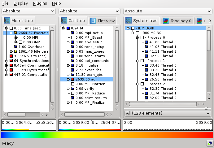
The CUBE-QT display has three tree browsers, each of them representing a dimension of the performance space (figure ). Per default, the left tree displays the metric dimension, the middle tree displays the program dimension, and the right tree displays the system dimension. The nodes in the metric tree represent metrics. The nodes in the program dimension can have different semantics depending on the particular view that has been selected. In Figure , they represent call paths forming a call tree. The nodes in the system dimension represent machines, nodes, processes, or threads from top to bottom.

CUBE display window

CUBE display window with expanded metric node ''Execution''

Each node is associated with a value, which is called the severity and is displayed simultaneously using a numerical value as well as a colored square. Colors enable the easy identification of nodes of interest even in a large tree, whereas the numerical values enable the precise comparison of individual values. The sign of a value is visually distinguished by the relief of the colored square. A raised relief indicates a positive sign, a sunken relief indicates a negative sign.

Users can perform two basic types of actions: selecting a node or expanding/collapsing a node. In the metric tree in figure , the metric Execution is selected. Selecting a node in a tree causes the other trees on its right to display values for that selection. For the example of figure , the metric tree displays the total metric values over all call tree and system nodes, the call tree displays values for the Execution metric over all system entities, and the system tree for the Execution metric and the adi call tree node. Briefly, a tree is always an aggregation over all selected nodes of its neighboring trees to the left.

Collapsed nodes with a subtree that is not shown are marked by a [+] sign, expanded nodes with a visible subtree by a [-] sign. You can expand/collapse a node by left-clicking on the corresponding [+]/[-] signs. Collapsed nodes have inclusive values, i.e., their severity is the sum of the severities over the whole collapsed subtree. For the example of Figure , the Execution metric value $ 3496.10 $ is the total time for all executions. On the other hand, the displayed values of expanded nodes are their exclusive values. E.g., the expanded Execution metric node in Figure shows that the program needed $ 2839.54 $ seconds for execution other than MPI.

Note that expanding/collapsing a selected node causes the change of the current values in the trees on its right-hand side. As explained above, in our example in Figure the call tree displays values for the Execution metric over all system entities. Since the Execution node is collapsed, the call tree severities are computed for the whole Execution metric's subtree. When expanding the selected Execution node, as shown in Figure , the call tree displays values for the Execution metric without the MPI metric.

GUI Components

The consists (from top to bottom) of

a menu bar,
three value mode combo boxes,
three resizable panes each containing some tabs,
three selected value information widgets,
a color legend, and
a status bar.

The three resizable panes offer different views: the metric, the call, and the system pane. You can switch between the different tabs of a pane by left-clicking on the desired tab at the top of the pane. Note that the order of the panes can be changed (see the description of the menu item Display Dimension order in Section ).

The metric pane provides only the metric tree browser. The call pane offers a call tree browser and a flat call profile. The system pane has a system tree browser. Tree browsers also provide a context menu.

Menu Bar

The menu bar consists of four menus: a file menu, a display menu, a plugin menu and a help menu. Some menu functions also have a keyboard shortcut, which is written besides the menu item's name in the menu. E.g., you can open a file with Ctrl+O without going into the menu. A short description of the menu items is visible in the status bar if you stay for a short while with the mouse above a menu item.

File: The file menu offers the following functions:
1. Open (Ctrl+O): Offers a selection dialog to open a CUBE file. In case of an already opened file, it will be closed before a new file gets opened. If a file got opened successfully, it gets added to the top of the recent files list (see below). If it was already in the list, it is moved to the top.
2. Save as (Ctrl+S): Offers a selection dialog to save a copy of a CUBE file. Opened CUBE file stays loaded in cube.
3. Close (Ctrl+W): Closes the currently opened CUBE file. Disabled if no file is opened.
4. Open external: Opens a file for the external percentage value mode (see Section ).
5. Close external: Closes the current external file and removes all corresponding data. Disabled if no external file is opened.
  
  %deprecated
6. Connect to trace browser: This menu item is only visible if a CUBE file with a corresponding statistics file, containing information about the most severe instances of certain performance patterns, is open and CUBE was configured for remote trace browsing. In this case, it offers to connect to a trace browser (i.e., Vampir or Paraver) to examine the behaviour of the program around the most severe pattern instances. For an in-depth explanation of this feature see subsection .
7. Settings: This menu item offers the saving, loading, and the deletion of settings. There are two types of settings, the global settings and the experiment settings.
  
  The global settings don't depend on the loaded cube file and are saved in a system specific format. These settings e.g. store the appearance of the application like the widget sizes, color and precision settings, the order of panes, etc. The default settings are automatically saved on exit and restored at startup, but it is also possible to save several settings under different names.
  
  The experiment settings depend on the loaded cube file. They allow to store e.g. which tree nodes are selected and which are expanded, the selected value mode etc. These settings are saved next to the opened cube file in the file cubebasename.ini. When saving experiment settings, the global settings are also saved in the .ini file. Like global settings, the default experiment settings are automatically saved and restored, but another behaviour may be chosen in the Settings menu. If the experiment settings toolbar is enabled, named settings can be selected and be saved in the .ini file.
8. Screenshot: The function offers you to save a screen snapshot in a PNG file. Unfortunately the outer frame of the main window is not saved, only the application itself.
9. Quit (Ctrl+Q): Closes the application.
10. Recent files: The last opened files are offered for re-opening, the top-most being the most recently opened one. A full path to the file is visible in the status bar if you move the mouse above one of the recent file items in the menu.
Display: The display menu offers the following functions:
1. Dimension order: As explained above, CUBE has three resizable panes. Initially the metric pane is on the left, the call pane is in the middle, and the system pane is on the right-hand side. However, sometimes you may be interested in other orders, and that is what this menu item is about. It offers all possible pane orderings. For example, assume you would like to see the metric and call values for a certain thread. In this case, you could place the system pane on the left, the metric pane in the middle, and the call pane on the right, as shown in Figure . Note that in panes to the left of the metric pane no meaningful valuescan be presented, since they miss a reference metric; in this case values are specified to be undefined, denoted by a ``-'' (minus) sign.
  
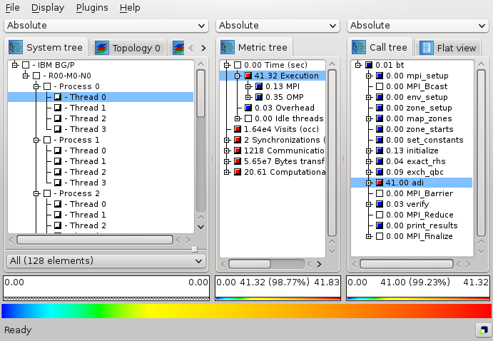  Modified pane order via the menu ''Display => Dimension order''
  
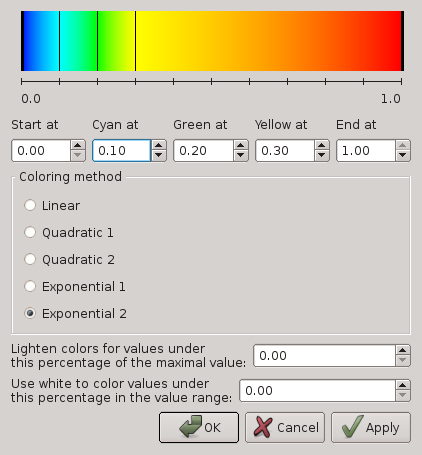  The color dialog opened via the menu ''Display => General coloring''
  
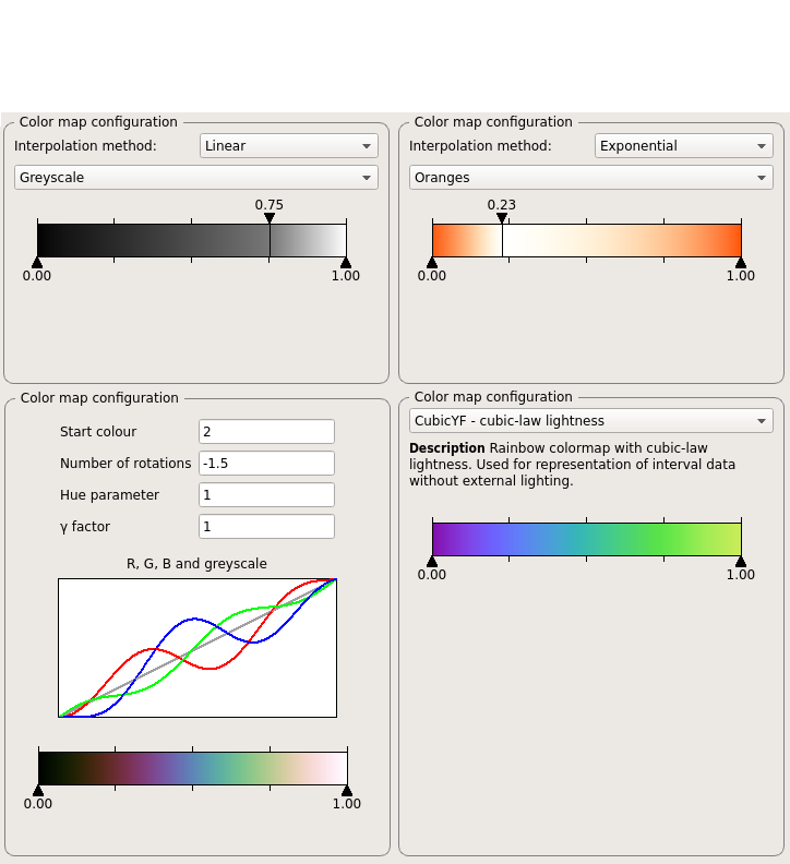  The examples of configuration for Advanced Color Maps. Upper row, starting from left: sequential, divergent; lower row, starting from left: cubehelix, improved rainbow.
2. General coloring: Allows for selection of color maps and changing of color settings in a new dialog. In the configuration dialog, the Ok button applies the settings to the display and closes the dialog, the Apply button applies the settings to the display, and Cancel cancels all changes since the dialog was opened (even if ``Apply'' was pressed in between) and closes the dialog.
  1. default: Default color map for Cube. The configuration dialog is show in Figure . At the top of the dialog you see a color legend with some vertical black lines, showing the position of the color scale start, the colors cyan, green, and yellow, and the color scale end. These lines can be dragged with the left mouse button, or their position can also be changed by typing in some values between (left end) and (right end) below the color legend in the corresponding spins.
    
    The different coloring methods offer different functions to interpolate the colors at positions between the data points specified above.
    
    With the upper spin below the coloring methods you can define a threshold percentage value between and , below which colors are lightened. The nearer to the left end of the color scale, the stronger the lightening (with linear increase).
    
    With the spin at the bottom of the dialog you can define a threshold percentage value between and , below which values should be colored white.
  2. Advanced Color Maps Cube plugin which provides additional color maps. The configuration dialogs are presented in Figure . For every color map, the plot allows for change of data accepted by color map and one can do that using left and right marker, by dragging the marker or providing exact position through a double click near the marker value (new dialog will appear). The default color for values out of range is grey.
    One can change colors of scheme (for some color maps) and color for values out of range. Double mouse click on proper part of the plot opens a dialog with selection of RGB color. Additionally, one can adjust the plot marker or reset to default values through the context menu.
    Currently the plugin adds four different sets of color maps:
    1. Sequential: Scheme is defined by starting and ending color with linear or exponential interpolation between them. Predefined schemes provide simple interpolation from one color to pure white. Middle marker allows for subtle change of interpolation.
    2. Divergent: This scheme is defined by an interpolation from starting to ending color, but with a critical value between them, depicted with the pure white. The position of critical point can be set with the middle marker.
    3. Cubehelix: Scheme designed primarily for display of astronomical intensity images. The coloring is based on distribution from black to white, with R, G and B helixes giving additional deviations. Cubehelix is defined by four parameters:
      Start colour - starting value for color, floating-point number between 0.0 and 3.0. R = 1, G = 2, B = 0
      Rotations - floating-point number of R -> G -> B rotations from the start to the end. Negative value corresponds to negative direction of rotation.
      Hue - non-negative value which controls saturation of the scheme, with pure greyscale for hue equal to 0.
      Gamma factor - non-negative value which configures intensity of colours. Values below one emphasizes low intensity values and creates brighter color scheme. Values above one emphasizes high intensity values and generates darker color map.
      Reference: Green, D. A., 2011, `A colour scheme for the display of astronomical intensity images', Bulletin of the Astronomical Society of India, 39, 289.
    4. Improved rainbow colormap: Set of color maps based on original jet (rainbow) scheme, but with different lightness distribution. The goal behind these schemes is to provide map with more balanced perception, which is poor for original jet, mainly because of sharp changes in lightness. These maps doesn't provide any possibility for configuration.
      Reference: Perceptually improved colormaps, MATLAB Central
3. Precision: Activating this menu item opens a dialog for precision settings (see Figure ). Besides Ok and Cancel, the dialog offers an Apply button, that applies the current dialog settings to the display. Pressing Cancel undoes all changes due to the dialog, even if you already pressed Apply previously, and closes the dialog. Ok applies the settings and closes the dialog.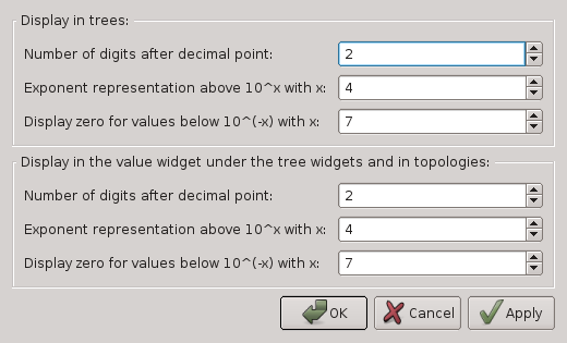
  
  Display => Precision
  
  It consists of two parts: precision settings for the tree displays, and precision settings for the selected value info widgets and the topology displays. For both formats, three values can be defined:
  1. Number of digits after the decimal point: As the name suggests, you can specify the precision for the fraction part of the values. E.g., the number 1.234 is displayed as 1.2 if you set this precision to 1, as 1.234 if you set it to 3, and as 1.2340 if you set it to 4.
  2. Exponent representation above with x: Here you can define above which threshold scientific notation should be used. E.g., the value 1000 is displayed as 1000 if this value is larger then 3 and as otherwise.
  3. Display zero values below $10^{-x}$ with x: Due to inexact floating point representation, it often happens that users wish to round down values very near by zero to zero. Here you can define the threshold below which this rounding should take place. E.g., the value 0.0001 is displayed as 0.0001 if this value is larger than 3 and as zero otherwise.
4. Trees: This menu item offers two sub-items:
  1. Font: Here you can specify the font, the font size (in pt), and the line spacing for the tree displays (see Figure ). The Ok button applies the settings to the display and closes the dialog, the Apply button applies the settings to the display, and Cancel cancels all changes since the dialog was opened (even if Apply was pressed in between) and closes the dialog.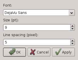
    
    The font dialog opened via the menu ''Display => Trees => Font''
  2. Selection marking: Here you can specify if selected items in trees should be marked by a blue background or by a frame.
5. Optimize width: Under this menu item CUBE offers widget rescaling such that the amount of information shown is maximized, i.e., CUBE optimally distributes the available space between its components. You can chose if you would like to stick to the current main window size, or if you allow to resize it.
Plugins: The plugin menu allows the user to define which plugins are laoded. For each loaded plugin, a submenu is added. The submenu contains a menu item to enable or disable the plugin and the plugin may add additional menu items.
1. Initial activation settings: Opens a dialog to define which plugins should be loaded.
Help: The help menu provides help on usage and gives some information about CUBE.
1. Getting started: Opens a dialog with some basic information on the usage of CUBE.
2. Mouse and keyboard control: Lists mouse and keyboard controls as given in Section .
3. What's this?: Here you can get more specific information on parts of the CUBE GUI. If you activate this menu item, you switch to the ``What's this?'' mode. If you now click on a widget, an appropriate help text is shown. The mode is left when help is given or when you press Esc.
  
  Another way to ask the question is to move the focus to the relevant widget and press Shift+F1.
4. About: Opens a dialog with release information.
5. Selected metric description: Opens a new window showing the description of the currently selected metric, equivalent to Online description in the metric tree context menu. Disabled if online information is unavailable.
6. Selected region description: Opens a new window showing the description of the currently selected region, equivalent to Online description in the call-tree context menu. Disabled if online information is unavailable.

Value modes

Each tree view has its own value mode combobox, a drop-down menu above the tree, where it is possible to change the way the severity values are displayed.

The default value mode is the Absolute value mode. In this mode, as explained below, the severity values from the CUBE file are displayed. However, sometimes these values may be hard to interpret, and in such cases other value modes can be applied. Basically, there are three categories of additional value modes.

The first category presents all severities in the tree as percentage of a reference value. The reference value can be the absolute value of a selected or a root node from the same tree or in one of the trees on the left-hand side. For example, in the Own root percent value mode the severity values are presented as percentage of the own root's (inclusive) severity value. This way you can see how the severities are distributed within the tree. All the value modes (Own root percent – System selection percent) fall into this category.

All nodes of trees on the left-hand side of the metric tree have undefined values. (Basically, we could compute values for them, but it would sum up the severities over all metrics, that have different meanings and usually even different units, and thus those values would not have much expressiveness.) Since we cannot compute percentage values based on undefined reference values, such value modes are not supported. For example, if the call tree is on the left-hand side, and the metric tree is in the middle, then the metric tree does not offer the Call root percent mode.
The second category is available for system trees only, and shows the distribution of the values within hierarchy levels. E.g., the Peer percent value mode displays the severities as percentage of the maximal value on the same hierarchy depth. The value modes (Peer percent – Peer distribution) fall into this category.
Finally, the External percent value mode relates the severity values to severities from another external CUBE file (see below for the explanation).

Depending on the type and position of the tree, the following value modes may be available:

Absolute (default): Available for all trees. The displayed values are the severity value as read from the cube file, in units of measurement (e.g., seconds). Note that these values can be negative, too, i.e., the expression ``absolute'' in not used in its mathematical sense here.
Own root percent:Available for all trees. The displayed node values are the percentage of their absolute values with respect to the absolute value of their root node in collapsed state.
Metric root percent: Available for trees on the right-hand side of the metric tree. The displayed node values are the percentage of their absolute values with respect to the absolute value of the collapsed metric root node. If there are several metric roots, the root of the selected metric node is taken. Note, that multiple selection in the metric tree is possible within one root's subtree only, thus there is always a unique metric root for this mode.
Metric selection percent: Available for trees on the right-hand side of the metric tree. The displayed node values are the percentage of their absolute values with respect to the selected metric node's absolute value in its current collapsed/expanded state. In case of multiple selection, the sum of the selected metrics' values for the percentage computation is taken.
Call root percent: Available for trees on the right-hand side of the call tree. Similar to the metric root percent, but the call tree root instead of the metric tree root is considered. In case of multiple selection with different call roots, the sum of those root values is considered.
Call selection percent: Available for trees on the right-hand side of the call tree. Similar to the metric selection percent, percentage is computed with respect to the selected call node's value in its current collapsed/expanded state. In case of multiple selections, the sum of the selected call values is considered.
System root percent: Available for trees on the right-hand side of the system tree. Similar to the call root percent, the sum of the inclusive values of all roots of selected system nodes are considered for percentage computation.
System selection percent:Available for trees on the right-hand side of the system tree. Similar to the call selection percent, percentage is computed with respect to the selected system node(s) in its current collapsed/expanded state.
Peer percent:For the system tree only. The peer percentage mode shows the percentage of the nodes' inclusive absolute values relative to the largest inclusive absolute peer value, i.e., to the largest inclusive value between all entities on the current hierarchy depth. For example, if there are 3 threads with inclusive absolute values 100, 120, and 200, then they have the peer percent values 50, 60, and 100.
Peer distribution:For the system tree only. The peer distribution mode shows the percentage of the system nodes' inclusive absolute values on the scale between the minimum and the maximum of peer inclusive absolute values. For example, if there are 3 threads with absolute values 100, 120 and 200, then they have the peer distribution values 0, 20 and 100.
External percent: Available for all trees, if the metric tree is the left-most widget. To facilitate the comparison of different experiments, users can choose the external percentage mode to display percentages relative to another data set. The external percentage mode is basically like the metric root percentage mode except that the value equal to 100% is determined by another data set.

Note that in all modes, only the leaf nodes in the system hierarchy (i.e., processes or threads) have associated severity values. All other hierarchy levels (i.e., machines, nodes and eventually processes) are only used to structure the hierarchy. This means that their severity is undefined—denoted by a ``-'' (minus) sign—when they are expanded.

System resource subsets

By default, all system resources (typically threads) are included when determining boxplot statistics. Other defined subsets can be chosen from the combobox below the boxplot, such as ``Visited'' threads which are only those threads that visited the currently selected callpath. The current subset is retained until another is explicitly chosen or a new subset is defined.

Additional subsets are defined from the system tree with the Define subset context menu using the currently selected threads via multiple selection (Ctrl+<left-mouse click>) or with the Find Items context menu selection option.

Tree browsers

A tree browser displays different hierarchical data structures in form of trees. Currently supported tree types are metric trees, call trees, flat call profiles, and system trees. The structure of the displayed data is common in all trees: The indentation of the tree nodes reflects the hierarchical structure. Expandable nodes, i.e., nodes with non-hidden children, are equipped with a [+]/[-] sign ([+] for collapsed and [-] for expanded nodes). Furthermore, all nodes have a color icon, a value, and a label.

The value of a node is computed, as explained earlier, basing on the current selections in the trees on the left-hand side and on the current value mode. The precision of the value display in trees can be modified, see the menu item Display Precision in Section . The color icon reflects the position of the node's value between $ 0.0 $ and a maximal value. These maximal value is the maximal value in the tree for the absolute value mode, or $ 100.0 $ otherwise. See the menu item Display General coloring in Section and the context menu item Min/max values in the context menu description below for color settings.

A label in the metric tree shows the metric's name. A label in the call tree shows the last callee of a particular call path. If you want to know the complete call path, you must read all labels from the root down to the particular node you are interested in. After switching to the flat profile view (see below), labels in the flat call profile denote methods or program regions. A label in the system tree shows the name of the system resource it represents, such as a node name or a machine name. Processes and threads are usually identified by a rank number, but it is possible to give them specific names when creating a CUBE file. The thread level of single-threaded applications is hidden. Multiple root nodes are supported.

After opening a data set, the middle panel shows the call tree of the program. However, a user might wish to know which fraction of a metric can be attributed to a particular region (e.g., method) regardless of from where it was called. In this case, you can switch from the call-tree view (default) to the flat-profile view (Figure ). In the flat-profile view, the call-tree hierarchy is replaced with a source-code hierarchy consisting of two levels: regions and their subroutines. Any subroutines are displayed as a single child node labeled Subroutines. A subroutine node represents all regions directly called from the region above. In this way, you are able to see which fraction of a metric is associated with a region exclusively, that is, without its regions called from there.

Tree displays are controlled by the left and right mouse buttons and some keyboard keys. The left mouse button is used to select or expand/collapse a node: You can expand/collapse a node by left-clicking on the attached [+]/[-] sign, and select it by left-clicking elsewhere in the node's line. To select multiple items, Ctrl+<left-mouse click> can be used. Selection without the Ctrl key deselects all previously selected nodes and selects the clicked node. In single-selection mode you can also use the up/down arrows to move the selection one node up/down. The right mouse button is used to pop up a context menu with node-specific information, such as online documentation (see the description of the context menu below).

CUBE flat profile

Each tree has its own context menu which can be activated by a right mouse click within the tree's window. If you right-click on one of the tree's nodes, this node gets framed, and serves as a reference node for some of the menu items. If you click outside of tree items, there is no refernce node, and some menu items are disabled.

The context menu consists, depending on the type of the tree, of some of the following items. If you move the mouse over a context menu item, the status bar displays some explanation of the functionality of that item.

Collapse all: For all trees. Collapses all nodes in the tree.
Collapse subtree: For all trees. Enabled only if there is a reference node. It collapses all nodes in the subtree of the reference node (including the reference node).
Collapse peers: For system trees only. Enabled only if there is a reference node. Collapses all peer nodes of the reference node, i.e., all nodes at the same hierarchy level.
Expand all: For all trees. Expands all nodes in the tree.
Expand subtree: For all trees. Enabled only if there is a reference node. Expands all nodes in the subtree of the reference node (including the reference node).
Expand peers: For system trees only. Enabled only if there is a reference node. Expands all peer nodes of the reference node, i.e., all nodes at the same hierarchy level.
Expand largest: For all trees. Enabled only if there is a reference node. Starting at the reference node, expands its child with the largest inclusive value (if any), and continues recursively with that child until it finds a leaf. It is recommended to collapse all nodes before using this function in order to be able to see the path along the largest values.
Dynamic hiding: Not available for metric trees. This menu item activates dynamic hiding. All currently hidden nodes get shown. You are asked to define a percentage threshold between and . All nodes whose color position on the color scale (in percent) is below this threshold get hidden. As default value, the color percentage position of the reference node is suggested, if you right-clicked over a node. If not, the default value is the last threshold. The hiding is called dynamic, because upon value changes (caused for example by changing the node selection) hiding is re-computed for the new values. In other words, value changes may change the visibility of the nodes.
1. Redefine threshold: This menu item is enabled if dynamic hiding is already activated. This function allows to re-define the dynamic hiding threshold as described above.
During dynamic hiding, for expanded nodes with some hidden children and for nodes with all of its children hidden, their displayed (exclusive) value includes the hidden children's inclusive value. The percentage of the hidden children is shown in brackets next to this aggregate value.
Static hiding: Not available for metric trees. This menu item activates static hiding. All currently hidden nodes stay hidden. Additionally, you can hide and show nodes using the now enabled sub-items:
1. Static hiding of minor values: Enabled only in the static hiding mode. As described under dynamic hiding, you are asked for a hiding threshold. All nodes whose current color position on the color scale is below this percentage threshold get hidden. However, in contrast to dynamic hiding, these hidings are static: Even if after some value changes the color position of a hidden node gets above the threshold, the node stays hidden.
2. Hide this: Enabled only in the static hiding mode if there is a reference node. Hides the reference node.
3. Show children of this: Enabled only in the static hiding mode if there is a reference node. Shows all hidden children of the reference node, if any.
Like for dynamic hiding, for expanded nodes with some hidden children and for nodes with all of its children hidden, their displayed (exclusive) value includes the hidden children's inclusive value. The percentage of the hidden children is shown in brackets next to this aggregate value.
No hiding: Not available for metric trees. This menu item deactivates any hiding, and shows all hidden nodes.
Find items: For all trees. Opens a dialog to get a regular expression from the user. If the user called the context menu over an item, the default text is the name of the reference node, otherwise it is the last regular expression which was searched for.

If select items is checked, items matching the regular expression also become selected.

If select items is unchecked, all non-hidden nodes whose names contain the given text are marked with a yellow background, and all collapsed nodes whose subtree contains such a non-hidden node by a light yellow background. The current node found, that is initialized to the first found node, is marked by a distinguished yellow hue.
Find next: For all trees. Changes the current found node to the next found node. If you did not start a search yet, then you are asked for the regular expression to search for.
Clear found items: For all trees. Removes the background markings of the preceding find items.
Define subset: Only for system tree. Uses the currently selected system resources (e.g., from a preceding Find items) to create a new subset of all system resources (typically threads) with the provided name. This is added to the combobox at the bottom of the system tree and boxplot statistics panes, and becomes the currently active subset for which statistics are calculated.
Info: For all trees (for call trees under Called region). Gives some short information about the reference node. Disabled if there is no reference node or if no information is available for the reference node.
Full Info: For metric tree and call tree only. In the case of metric tree it lists a complete information about the selected metric. One gets information about display and unique name, data type, unit of measurements, kind of metric and CubePL expression if the metric is derived.

In the case of call tree it lists a complete available information about the selected call path. One gets information about call path id (to use it with command line tools like cube_dump), region begining line, region ending line, region module, url with the online help and finally description of the region.

Disabled if not clicked over metric item or call path item.
Online description: For metric trees and flat call profiles (for call trees see under Called region). Shows some (usually more extensive) online description for the reference node. For example, metrics might point to an online documentation explaining their semantics, or regions representing library functions might point to the corresponding library documentation. Disabled if there is no reference node or if no online information is available.
Location: For flat profiles only. Disabled if there is no reference node. Displays information about the module and position within the module (line numbers) where the method is defined.
Source code: For flat call profiles only (for call trees see Call site and Called region below). Disabled if there is no reference node. Opens an editor for displaying, editing, and saving the source code of the method/region to which the reference node refers. The begin and the end of the method/region are highlighted. If the specified source file is not found, you are asked to choose a file to open.

The file is in a read-only mode per default. If you wish to edit the text, please uncheck the Read only box in the bottom left corner. For keyboard and mouse control, see Section .

The item main with 1000 iteration is marked as a loop. The aggregated view on the right is the result of selecting ''Hide iterations''.
Hide iterations: Only visible for calltree items that are recognized or manually defined as loop (see "Set as loop" below). By activating, all children of the loop are hidden. The grandchildren are shown and its values for the different iterations are aggregated (see Figure ).
Call site: For call trees only. Enabled only if there is a reference node. Offers information about the caller of the reference node.
1. Location: Displays information about the module and position within the module (line numbers) of the caller of the reference node.
2. Source code: Opens an editor for displaying, editing, and saving the source code where the call for which the reference node stays for happens. The begin and the end of the relevant source code region are highlighted. If the specified source file is not found, you are asked to chose a file to open.
3. Set as loop: Marks the selected tree item as loop. All subitems are treated as iterations. An additional context menu item "Hide iterations" appears.
Called region: For call trees only. Enabled only if there is a reference node. Offers information about the reference node.
1. Info: Gives some short information about the reference node.
2. Online description: Shows some (usually more extensive) online description for the reference node. Disabled if no online description is available.
3. Location: Displays information about the module and position within the module (line numbers) where the callee method of the reference node is defined.
4. Source code: Opens an editor for displaying, editing, and saving the source code of the callee of the reference node. Begin and end of the relevant region are highlighted. If the specified source code does not exists, you are asked to choose a file to open.
Min/max values: Not for metric trees. Here you can activate and deactivate the application of user-defined minimal and maximal values for the color extremes, i.e., the values corresponding to the left and right end of the color legend. If you activate user-defined values for the color extremes, you are asked to define two values that should correspond to the minimal and to the maximal colors. All values outside of this interval will get the color gray. Note that canceling any of the input windows causes no changes in the coloring method. If user-defined min/max values are activated, the selected value information widget (see Section ) displays a (u)'' foruser-defined'' behind the minimal and maximal color values.
Statistics: Only available if a statistics file for the current CUBE file is provided. Displays statistical information about the instances of the selected metric in the form of a box plot. For an in-depth explanation of this feature see subsection .
Max severity in trace browser: Only available for metric and call trees and only if a statistics file providing information about the most severe instance(s) of the selected metric is present. If CUBE is already connected to a trace browser (via File Connect to trace browser), the timeline display of the trace browser is zoomed to the position of the occurrence of the most severe pattern so that the cause for the pattern can be examined further. For a more detailed explanation of this feature see subsection .
Cut all tree: For call trees only. Enabled only if clicked over item in call tree. Offers different modification possibilities:
1. Set as root: Removes all call path above the selected item and sets selected call path as a root node.
2. Prune element: Removes the selected item and all its children. Its inclusive value will be added then to the exclusive value of its parent.
3. Set as leaf: Removes all children of its element and add their inclusive values to its exclusive value.
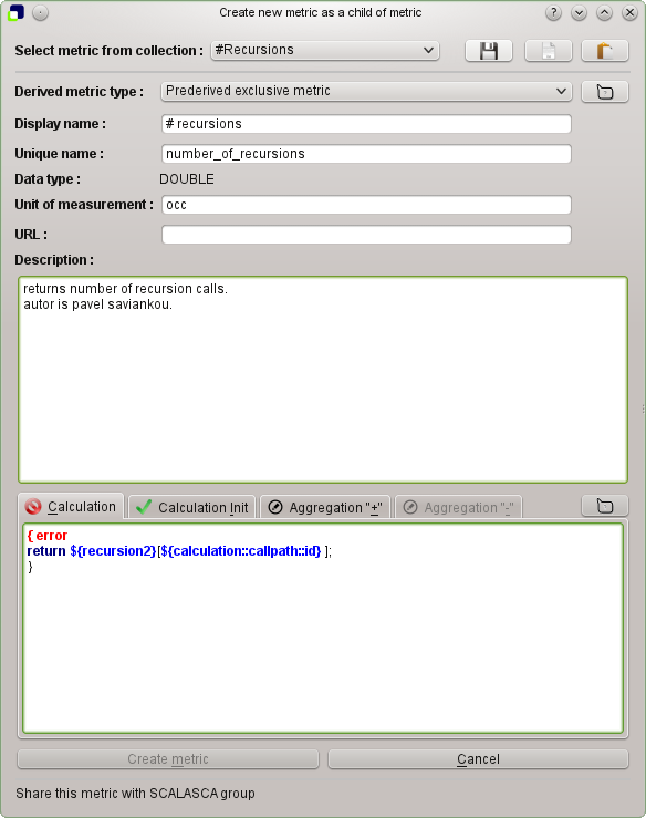
Create derived metric (as root or a child) For metric tree only. It offers a dialog to create a new derived metric as a root metric if clicked over an empty part of window or selected via submenu as a root. An it creates the new metric as a child metric if clicked over another metric or selected via submenu as a child.

Create derived metric

Documentation about derived metrics see in
Some details about the fields in the dialog:
1. Select metric from collection: Provides a list of predefined derived metric, which might be helpful for the analysis.
2. Derived metric type: Selects the type of the derived metrics. Available are : Postderived metric, Prederived exclusive metric and Prederived inclusive metric.
3. Display name: Sets the display name of the metric in the metric tree.
4. Unique name: Sets the unique name of the metric. There is no check done if another metric is present with the same unique name.
5. Data type : For derived metrics it is preselected and is always DOUBLE.
6. Unit of measurement: Selects a unit of measurement. It is a user defined string.
7. URL: Selects a URL with the documentation about this metric.
8. Description: Describes a metric.
9. Calculation: Field where one enters the CubePL expression for the derived metric. Automatic syntax check is done. If there is a syntax error, dialog highlights the place of the error and gives an error message.
10. Calculation Init: Field where one enters the initialisation CubePL expression for the derived metric,which is executed only once after metric creation.
  
  Automatic syntax check is done. If there is a syntax error, dialog highlights the place of the error and gives an error message.
11. Aggregaton "+":Prederived metrics can specify an expression for the operator "+" in the aggregation formula. In this field one can redefine it.
  
  Automatic syntax check is done. If there is a syntax error, dialog highlights the place of the error and gives an error message.
12. Calculation "-": Prederived inclusive metric can specify an expression for the operator "-" in the aggregation formula. In this field one can redefine it.
  
  Automatic syntax check is done. If there is a syntax error, dialog highlights the place of the error and gives an error message.
13. Create metric - closes dialog and creates metric with parameters, set in this dialog. Enabled if syntax is OK type of metric is selected and fields Unique name Display name are set.
14. Cancel - closes dialog without creating any metric.
15. Share this metric with SCALASCA group - Offers you to sent the metric definition via email to the SCALASCA group, so it might be included into the library of derived metrics in the future releases. Enabled only if definition of metric is valid.
To simplify the creation of a derived metric a little bit there is a way to fill the fields of this dialog automatically.

If one prepares a file with the following syntax one can select it and open "drop" on dialog via drag'n'drop, or copy its content into clipboard and paste in the dialog.

Example of a syntax of this file:
metric type: postderived

display name: Average execution time

unique name: kenobi

uom:sec

url: https://scalasca.org/documentation.html#kenobi

description:Calculates an average execution time

#

# Here is the Kenobi metric

#

cubepl expression: metric::time(i)/metric::visits(e)

cubepl init expression:

cubepl plus expression: arg1 + arg2

cubepl minus expression: arg1 - arg2

metric type can have values: postderived, prederived_exclusive or prederived_inclusive.
Remove metric For metric tree only. Removes metric from the metric tree.
Edit metric For metric tree only. It offers a dialog to edit expressions (standard, initialisation, aggregation) of a derived metric. Enabled if clicket metric is a derived metric. Window for editing is same like in "Create derived metric" case.
Sort by value (descending): For flat call profiles only. Sorts the nodes by their current values in descending order. Note that if an item is expanded its exclusive value is taken for sorting, otherwise its inclusive value.
Sort by name (ascending): For flat call profiles only. Sorts the nodes alphabetically by name in ascending order.

Selected value info

Below each pane there is a selected value information widget. If no data is loaded, the widget is empty. Otherwise, the widget displays more extensive and precise information about the selected values in the tree above. This information widget and the topologies may have different precision settings than the trees, such that there is the possibility to display more precise information here than in the trees (see Section , menu Display Precision).

The widget has a 3-line display. The first line displays at most 4 numbers. The left-most number shows the smallest value in the tree (or $ 0.0 $ in any percentage value mode for trees, or the user-defined minimal value for coloring if activated), and the right-most number shows the largest value in the tree (or $ 100.0 $ in any percentage value mode in trees, or the user-defined maximal value for coloring if activated). Between these two numbers the current value of the selected node is displayed, if it is defined. Additionally, in the absolute value mode it is followed by the percentage of the selected value on the scale between the minimal and maximal values, shown in brackets. Note that the values of expanded non-leaf system nodes and of nodes of trees on the left-hand side of the metric tree are not defined. If the value mode is not the absolute value mode, then in the second line similar information is displayed for the absolute values in a light gray color.

In case of multiple selection, the information refers to the sum of all selected values. In case of multiple selection in system trees in the peer distribution and in the peer percent modes, this sum does not state any valuable information, but is displayed for consistency reasons.

If the widget width is not large enough to display all numbers in the given precision, then a part of the number displays get cut down and a `` $\ldots$ '' indicates that not all digits could be displayed.

Below these numbers, in the third line, a small color bar shows the position of the color of the selected node in the color legend. In case of undefined values, the legend is filled with a gray grid.

Color legend

By default, the colors are taken from a spectrum ranging from blue over cyan, green, and yellow to red, representing the whole range of possible values. You can change the color settings in the menu,Display General coloring, see Section . Exact zero values are represented by the color white (in topologies you can decide whether you would like to use white or the minimal color, see Section , menu Topology).

Status Bar

The status bar displays some status information, like state of execution for longer procedures, hints for menus the mouse pointing at etc.

The status bar shows the most recent log message. By clicking on it, the complete log becomes visible.

Plugins

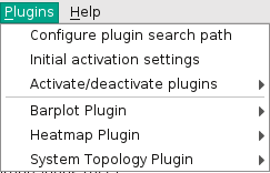
The features of cube can be extended using plugins. There is a set of predefined plugins which are described in the following sections. Before a cube file is loaded, the Plugin menu only contains the menu items "Configure plugin search path" and "Initial activation settings".

plugin menu

By Selecting the second item, a dialog is created which lists all available plugins (see Figure ).

plugin settings dialog

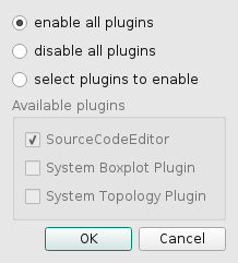
You may enable or disable all plugins, or select individual plugins that will be activated or deactivated. After loading a cube file, all suitable plugins are activated. Each plugin may add a submenu (see Figure ) to the Plugins menu.

Cube searches for plugins in the directory "cube-plugins/" below the installation directory. This is the place where the predefined plugins are installed. If the environment variable CUBE_PLUGIN_DIR contains a colon or semicolon separated list of pathes, these pathes are prepended to the default search path.

plugin search path dialog

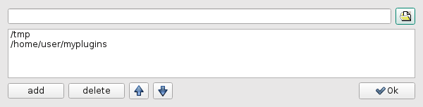
Selecting "Configure plugin search path" of the plugin menu shows a dialog (see Figure ), which allows to prepend additional search pathes. The directory icon on the right opens a file browser whose selection is added to the input line on top and which is added to the path with the "add" button.

Tree Item Marker

A plugin may define one or more tree item marker to tag items of interest.

Tree items are marked in different ways:

Items with a colored background show that a plugin has set a marker
Items with a colored frame indicate that a collapsed child has been marked.
Items with a black frame indicate that there are several collapsed children with different marker.
Items with a dotted frame show a dependency. A marked item of the right neighbor tree depends on this item. The dependent item is only marked, if the dotted item is selected.

tree item marker

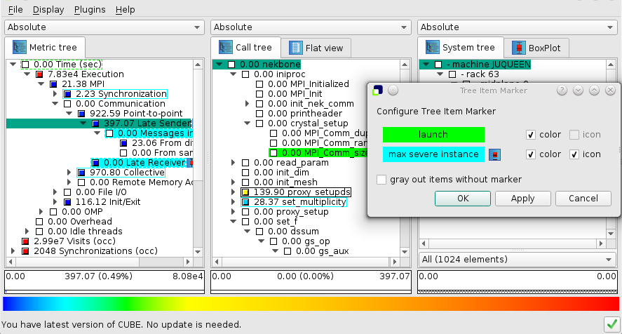
The figure shows two plugins which define marker. The Statistic Plugin marks all items with information about the most severe instances with a blue background and an icon. The Launch Plugin uses green marker and does not define an icon. Both of them use marker for items of the system tree and for items of the call tree that depend on items of the system tree.

The Tree Item Marker dialog (see figure ) allows the user to change the color of each marker, to disable the drawing of colors or icons and to emphasize the marked items by graying out the other items.

TopologyPlugin

In many parallel applications, each process (or thread) communicates only with a limited number of processes. The parallel algorithm divides the application domain into smaller chunks known as sub-domains. A process usually communicates with processes owning sub-domains adjacent to its own. The mapping of data onto processes and the neighborhood relationship resulting from this mapping is called virtual topology. Many applications use one or more virtual topologies specified as multi-dimensional Cartesian grids.

Another sort of topologies are physical topologies reflecting the hardware structure on which the application was run. A typical three-dimensional physical topology is given by the (hardware) nodes in the first dimension, and the arrangement of cores/processors on nodes in further two dimensions.

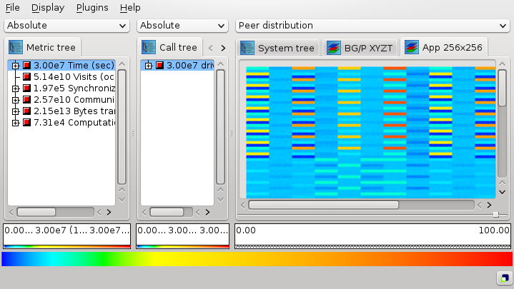
The CUBE display supports multi-dimensional Cartesian grids, where grids with high dimensionality can be sliced or folded down to two or three dimensions for presentation. If the currently opened cube file defines one or more such topologies, separate tabs are available for each using the topology name when one is provided. The topology display shows performance data mapped onto the Cartesian topology of the application. The corresponding grid is specified by the number of dimensions and the size of each dimension. Threads/processes are attached to the grid elements, as specified by the CUBE file. Not all system items have to be attached to a grid element, and not every grid element has a system item attached. An example of a three-dimensional topology is shown on Figure . Note that the topology toolbar is enabled when a topology is available to be displayed.

Topology Displays

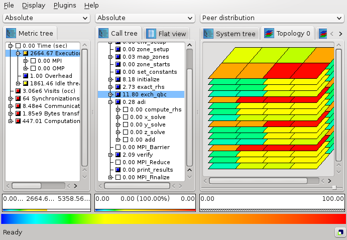
The Cartesian grid is presented by planes stacked on top of each other in a three dimensional projection. The number of planes depends on the number of dimensions in the grid. Each plane is divided into tiles (typically shown as rombi). The number of tiles depends on the dimension size. Each tile represents a system resource (e.g., a process) of the application and has a coordinate associated with it.

The current value of each grid element (with respect to the selections on the left-hand side and to the current value mode) is represented by coloring the grid element. Coloring is based on a value scale from $ 0.0 $ to $ 100.0 $ . Grid elements without having a system item attached to it are colored gray. See Section (menu Topology) for further topology-specific coloring settings. For example, the upper topology in Figure is drawn wit black lines, the 2D topology in Figure is drawn without lines.

Topology Displays

If the selected system item occurs in the topology, it is marked by an additional frame and by additional lines at the side of the plane which contains the corresponding grid point, such that the selected item's position is also visible if the corresponding plane is not completely visible.

If zooming into planes is enabled, the plane containing the recently selected item is selected and the plane distance is adjusted to show this plane complely.

Selecting a collapsed tree in the system tree selects all its children in the topology view.

Besides the functions offered by the topology toolbar (see ), the following functionality is supported:

Item selection: You can change the current system selection by left-clicking on a grid element which has a system item assigned to it (resulting in the selection of that system item). Multiple items may be selected or deselected by holding down the Ctrl key while clicking on an item.
Info: By right-clicking on a grid element, an information widget appears with information about the system item assigned to it. The information contains
- the coordinate of the grid point in each topology dimension,
- the hardware node to which the attached system item belongs to,
- the system item's name,
- its MPI rank,
- its identifier,
- and its value, followed by the percentage of this value on the scale between the minimal and maximal topology values.
Rotation about the x and y axes: can be done with left-mouse drag (click and hold the left-mouse button while moving the mouse).
Increasing/decreasing the distance between the planes: with Ctrl+<left-mouse drag>
Moving the whole topology up/down/left/right: with Shift+<left-mouse drag>

Topology mapping panel

If the number of topology dimensions is larger than three, the first three dimensions are shown and an additional control panel appears below the displayed topology. This panel allows rearranging topology dimensions on the x, y and z axes, as well as slicing or folding of higher dimensionality topologies for presentation in three or fewer dimensions.

Rearranging topology dimensions is achieved simply by dragging the topology dimension labels to the desired axis. When dragged on top of an existing topology dimension label, the two are exchanged.

When slicing, select up to three of the dimensions to display completely and choose one element of each of the remaining dimensions. The example in Figure shows a topology with 4 dimensions (32x16x32x4) labelled X, Y, Z and T. The first element of the 4th dimension (T) is automatically selected. By clicking on the button above the T, an index in this dimension from 0 to 3 can be chosen. If the index is set to all, the selection becomes invalid until an index of another dimension is selected.

4-dimensional example

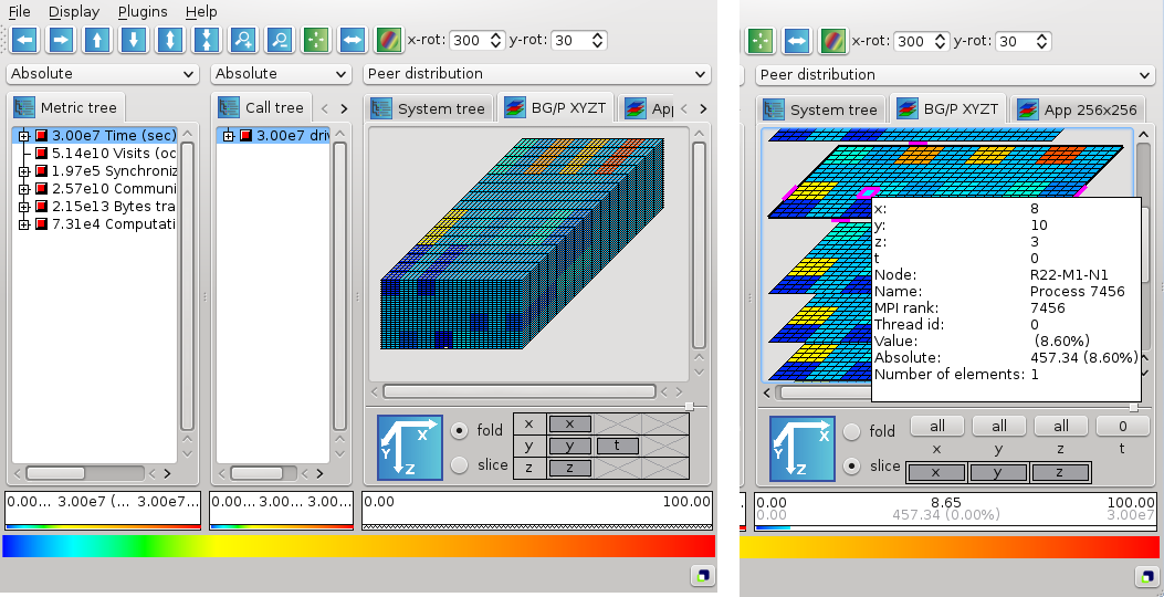
Alternatively, the folding mode can be activated by clicking on the fold button. This mode is available for topologies with four to six dimensions and allows to display all elements by folding two dimensions into one. Every dimension appears in a box, with can be dragged into one of the three container boxes for the displayed dimensions x, y and z. In folding mode, the color of the inner borders is changed into gray. The black bordered rectangles show the element borders of each of the three displayed dimensions.

The right image in Figure shows the folding of dimension Z with dimension T. One element with index (0,0,1,3) has been selected by clicking with the right mouse button into it. All elements inside the black rectancle around the selection belong to Z index one. The gray lines devide the rectangle into four elements which correspond to the elements of dimension T with index 0 to 3.

TopologyPlugin

Topology: The topology menu offers the following functions related to the topology display described in Section :

Item coloring: Offers a choice how zero-valued system nodes should be colored in the topology display. The two offered options are either to use white or to use white only if all system leaf values are zero and use the minimal color otherwise.
Line coloring: Allows to define the color of the lines in topology painting. Available colors are black, gray, white, or no lines.
Toolbar: This menu item allows to specify if the topology toolbar buttons should be labeled by icons, by a text description, or if the toolbar should be hidden. For more information about the toolbar see Section .
Show also unused hardware in topology: If not checked, unused topology planes, i.e., planes whose grid elements don't have any processes/threads assigned to, are hidden. Unused plane elements, if not hidden, are colored gray.
Topology antialiasing: If checked, anti-aliasing is used when drawing lines in the topologies.
Zoom into current plane: If checked, the plane containing the recently selected item is shown completely. It is never covered by a neighbor plane.

Toolbar

The system pane may contain topology displays if corresponding data is specified in the CUBE file. Basically, a topology display draws a two- or three-dimensional grid, in the form of some planes placed one above the other. Each plane consists of a two-dimensional grid of processes or threads.

The toolbar is enabled only if the system pane shows a topology display, and it offers functions to manipulate the display of the above grid planes. The toolbar can be labeled by icons, by text, or it can be hidden, see menu Topology Toolbar in Section . The toolbar buttons have tool tips, i.e., a short description pops up if the toolbar is enabled and you move the mouse above a button.

The functions are the following, listed from the left to the right in the topology toolbar:

Move left: Moves the whole topology to the left.
Move right: Moves the whole topology to the right.
Move up: Moves the whole topology upwards.
Move down: Moves the whole topology downwards.
Increase plane distance: Increase the distance between the planes of the topology.
Decrease plane distance: Decrease the distance between the planes of the topology.
Zoom in: Enlarge the topology.
Zoom out: Scale down the topology.
Reset: Reset the display. It scales the topology such that it fits into the visible rectangle, and transforms it into a default position.
Scale into window: It scales the topology such that it fits into the visible rectangle, without transformations.
Set minimum/maximum values for coloring: Similarly to the functions offered in the context menu of trees (see Section ), you can activate and deactivate the application of user-defined minimal and maximal values for the color extremes, i.e., the values corresponding to the left and right end of the color legend. If you activate user-defined values for the color extremes, you are asked to define two values that should correspond to the minimal and to the maximal colors. All values outside of this interval will get the color gray. Note that canceling any of the input windows causes no changes in the coloring method. If user-defined min/max values are activated, the selected value information widget displays a (u)'' foruser-defined'' behind the minimal and maximal color values.
x-rotation: Rotate the topology cube about the x-axis with the defined angle.
y-rotation: Rotate the topology cube about the y-axis with the defined angle.
Dimension order for the topology displays: This button no longer exists, but formerly allowed the order of topology dimensions to be adjusted: this is now done with the control panel at the bottom of the topology pane.

Using the grip at the left of the toolbar, it can be dragged to another position or detached entirely from the main window. The toolbar can also be closed after a right-click in the grip.

BarplotPlugin

BARPLOT plugin is a CUBE plugin that plots vertical bar graph for the CUBE file which has iterations. Horizontal axis shows different iterations being compared and on vertical axis, several operations can be used to represent the value. The User can apply different metrics and call paths on the bar graph.

Basic Principles

As a start point, it should be mentioned that BARPLOT works only on a CUBE file that has iterations. For those files which have not, user would face the warning on the terminal : "No iterations for Barplot" and the plugin will not be shown.

By loading the plugin, on system dimension, the corresponding tab, Barplot, will be added. In the Barplot tab, the user can select different operations and assign desired color to them. Figure displays a view of it.

BARPLOT display window

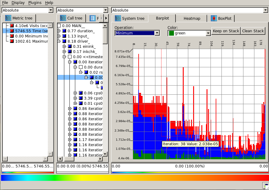
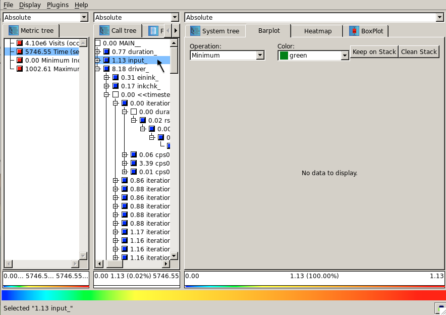
User can select different metrics such as Visits and Time, by clicking on them in metric dimension. In addition, it is possible to get a BARPLOT for different call paths of iterations, via clicking on them. However, for call paths that are not located in iterations, like input_in in figure , no bar graph is displayed and user face the message "No data to display" on the window.

No data to display

Furthermore, the values on BARPLOT, can be evaluated in Inclusive and Exclusive manner. Therefore, user can easily collapse the tree on call path and click on the desired path to get the exclusive value of it.

Additionally, the exact calculated values can be seen by clicking left button of mouse on the desired position on the graph, a tooltip would display a value corresponding to the iteration.

In a situation that user needs to store the graph, it is just needed to do right click on a graph, and select "Save as image", then the Save dialog will be opened to specifying the path and name of the PNG file.

Toolbar

On the top of the Barplot space, there is a toolbar that allows user to specify the kind of an operation and its color(Figure ).

BARPLOT toolbar

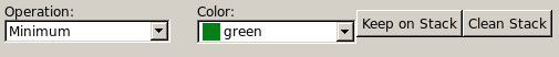
By operation item, the user can select different operations, Minimum, Maximum, Average, Median, 1st Quartile and 3rd Quartile or the combination of Maximum, Minimum and Average. This provides the situation for the user to have different values for comparing at one time. These operations are done on all threads in each iterations. For instance, by Minimum operation, the minimum value among the existing threads for each iteration, is calculated and plotted. They are kind of statistical measurements.

Color item offers a color for an operation, however for each operation, a default color is assigned automatically. By changing the operation, corresponding color will be shown on color combo box. In a situation that different bar graphs are overlaid on each other, each graph will be shown by different color in order to distinguish various graphs.

In addition to above items, two buttons are also designed to manage the order of the bar graphs.

Keep on Stack: It is possible that user intents to compare different graphs by laying them on each other. For this matter, a push-button keep on stack is defined. Generally, by clicking on each call path or metric, a responding graph is replaced the previous one in the stack. In a situation, that the user intends to compare the next graph by the existing one, at one time, it is needed to click on the button keep on the stack, then the next graph will be added over the previous one, or in another words, it is overlaid on the last graph. If its values are less than the previous graph, user can see two graphs by different colors that help him/her in comparing, and in a situation that new values are greater than previous one, the new one will cover the previous with fresh color. Therefore, for keeping the top row of the stack, the user should click on the keep the stack button, otherwise the coming values will replace the last one.

Clean Stack: By clicking this button, all displayed graphs, are erased and the stack will be empty.

Menu Bar

Plugin menu offers the general function to enable or disable a plugin, and specific functions for each plugin. Barplot plugin provides the following functions in two areas, Measurement Customization and Threads Ruler Customization(Fiqure ).

BARPLOT menu

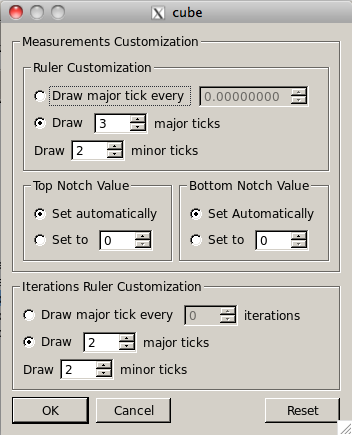
Ruler Customization: User can modify the number of major and minor ticks of the ruler on vertical axis. For adjusting the major vertical ticks, user can set the drawing intervals or the number of ticks. By specifying the number of major ticks, the length of the vertical axis will be divided to the specified number and major ticks are drawn by length longer than minor ticks. Then in each divided length, if there is enough space, the specified number of minor ticks will be displayed. It is possible that the user set major ticks by interval. In order to do that, select the major ticks by interval option, and set the interval value. Therefore, after each interval, one major tick will be drawn.

Top Notch Value: The value of the top notch on a vertical axis can be altered by user as well as automatically. Therefore, due to scale issue, it can affect on the drawing of the graph.

Button Notch Value: The value of the button notch on a vertical axis can be altered by user as well as automatically. Therefore, due to scale issue,it can affect on the drawing of the graph.

Iterations Ruler Customization: User can modify the number of major and minor ticks of the ruler on horizontal axis. For adjusting the major horizontal ticks, user can set the drawing intervals or the number of ticks. By specifying the number of major ticks, the width of the horizontal axis will be divided to the specified number and major ticks are drawn by length longer than minor ticks. Then in each divided length, if there is enough space, the specified number of minor ticks will be displayed. It is possible that the user set major ticks by interval of iterations. In order to do that, select the major ticks by interval option, and set the interval. Therefore, after each specified number of iterations, one major tick will be drawn.

HeatmapPlugin

HEATMAP plugin is a CUBE plugin that represents the value of the thread in each iteration, as colors. The User can apply different metrics and call paths on heatmap graph.

Basic Principles

As a start point, it should be mentioned that HEATMAP works only on CUBE file that has iterations. For those files which have not, user would face the warning on the terminal : "No iterations for Heatmap" and the plugin will not be shown.

By loading the plugin, on system dimension, the corresponding tab, Heatmap, will be added. Figure displays a view of it.

HEATMAP display window

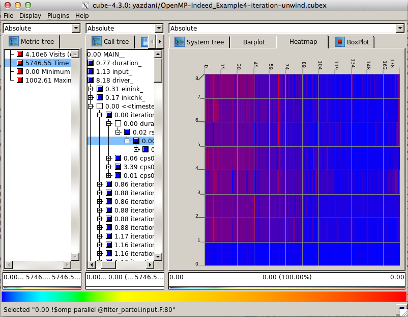
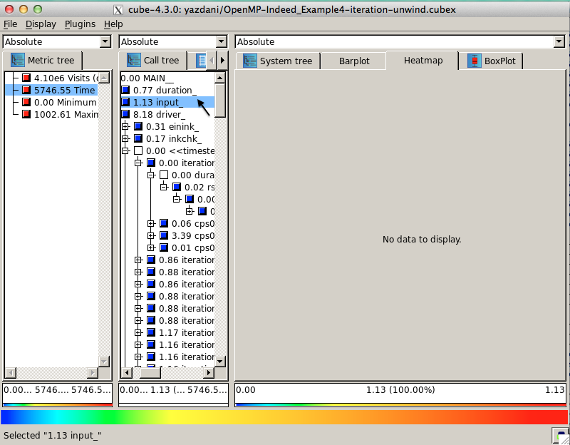
User can select different metrics such as Visits and Time, by clicking on them in metric dimension. In addition, it is possible to get a HEATMAP for different call paths of iterations, via clicking on them. However, for call paths that are not located in iterations, like input_in figure , no heatmap graph is displayed and user face the message "No data to display" on a window.

No data to display

Furthermore, the values on HEATMAP, can be evaluated in Inclusive and Exclusive manner. Therefore, user can easily collapse the tree on call path and click on the desired path to get the exclusive value of it.

Additionally, the exact calculated values can be seen by clicking left button of mouse on the desired position on the graph, a tooltip would display a value corresponding to the iteration.

In a situation that user needs to store the graph, it is just needed to do right click on a graph, and select "Save as image", then the Save dialog will be opened to specifying the path and name of the PNG file.

Menu Heatmap

Plugin menu offers the general function to enable or disable a plugin, and specific functions for each plugin. Heatmap plugin provides the following functions in two areas, horizontal tick and vertical ticks(Fiqure ).

HEATMAP menu

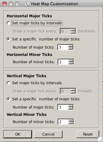
Horizontal ticks: For adjusting the major horizontal ticks, user can set the drawing intervals or the number of ticks. By specifying the number of major ticks, the width of the horizontal axis will be divided to the specified number and major ticks are drawn by length longer than minor ticks. Then in each divided length, if there is enough space, the specified number of minor ticks will be displayed.

Also, it is possible that the user set major ticks by interval of iterations. In order to do that, select the major ticks by interval option, and set the interval. Therefore, after each specified number of iterations, one major tick will be drawn.

Vertical ticks: For adjusting the major vertical ticks, user can set the drawing intervals or the number of ticks. By specifying the number of major ticks, the length of the vertical axis will be divided to the specified number and major ticks are drawn by length longer than minor ticks. Then in each divided length, if there is enough space, the specified number of minor ticks will be displayed.

Also, it is possible that the user set major ticks by interval of threads. In order to do that, select the major ticks by interval option, and set the interval. Therefore, after each specified number of threads, one major tick will be drawn.

SystemBoxplotPlugin

This plugin adds a boxplot statistics display tab next to the system tree tab. It shows a box-and-whisker distribution of metric severity values for the currently active subset of system resources (typically threads). The active subset is changed via the combobox menu at the bottom of the pane, and the y-axis scale is adjusted via the display mode combobox at the top of the pane.

The vertical whisker ranges from the smallest value (minimum) and to the largest value (maximum), while the bottom and top of the box mark the lower quartile (Q1) and upper quartile (Q3). Within the box, the bold horizontal line represents the median (Q2) and the dashed line the mean value.

To see the statistics as numeric values in a separate window, use <left-mouse click> inside the chart. Zooming into the boxplot is done with <left-mouse drag> from top to bottom, and reset with a <middle-mouse click> inside the chart.

%deprecated

Features enabled through statistic files

In this section we will explain two features – namely the display of statistical information about performance patterns which represent performance problems and the display of the most severe instances of these patterns in a trace browser – which both are only available if a statistic file for the currently opened CUBE file is present. Currently, such a statistic file can be generated by the SCOUT analyzer . The file format of statistic files is described in the Appendix .

For CUBE to recognize the statistic file, it must be placed in the same directory as the CUBE file. The basename of the statistic file should be identical to that of the CUBE file, but with the suffix .stat. For example, when the CUBE file is called trace.cubex, the corresponding statistic file is called trace.stat.

Statistical information about performance patterns

If a statistic file is provided, you can view statistical information about one or multiple patterns (for example in order to compare them). This is done by selecting the desired metrics in the metric tree and then selecting the Statistics menu item in the context menu. This brings up the box plot window as shown in Figure .

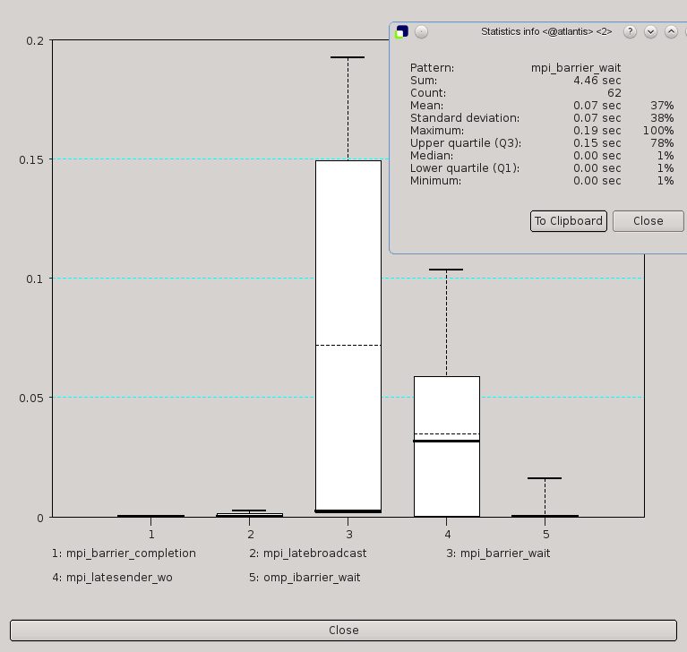
Screenshot of a box plot as shown by CUBE displaying statistical information about the selected patterns. The additional window on the top right displaying the exact values of the statistics.

The box plot shows a graphical representation of the statistical data of the selected patterns. The slender black lines on the top and the bottom designate the maximum and the minimum measured severity of the pattern, respectively. The lower and the upper borders of the white box indicate the values of the 25% and 75% quantile. The thick line inside the box represents the median of the values, while the dashed line indicates the mean.

There are two ways of interacting with the box plot. You can zoom to a certain interval on the y-axis by clicking on a position with the height of the desired maximal or minimal value and by consecutively dragging the mouse to a position with the height of the corresponding other extreme value. You can reset the view (i.e., to undo all zooming) by clicking the middle mouse button somewhere on the box plot.

If you are interested in more precise values for the severity statistics of a certain metric, you can click somewhere in the column of the desired metric, which will yield a small window (as shown in the top right corner of Figure ) displaying the exact values of the statistics.

Display of most severe pattern instances using a trace browser

If a statistic file also contains information about the most severe instances of certain patterns, CUBE can be connected to a trace browser (currently Vampir and Paraver are supported) in order to view the state of the program being analyzed at the time this most severe pattern instance occurred. For collective operations, the most severe instance is the one with the largest sum of the waiting times of all processes, which is not necessarily the one with the largest maximal waiting time of each individual process.

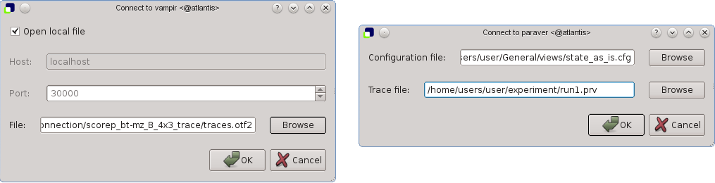
The dialog windows for a connection to Vampir and to Paraver

To use this feature, you first have to connect to a trace browser by using the Connect to menu item of the Vampir Plugin or Paraver Plugin submenu of the Plugin menu. This will open one of the two dialog windows shown below.

For Vampir, you have to specify the host name and port of the Vampir server you want to connect to and the path of the trace file you want to load. This will launch the Vampir client (if it is correctly configured) and load the specified trace file. To configure Vampir so that it can be started automatically by CUBE, a service file com.gwt.vampir.service, describing the path to your Vampir client executable must be placed under (/usr/share/dbus-1/service) or ${HOME}/.local/share/dbus-1/services. This service file must be exactly as shown below, with the exception that Exec should point to your Vampir client executable.

[D-BUS Service]
Name=com.gwt.vampir
Exec=/private/utils/bin/vng

An example of the com.gwt.vampir.service file

For Paraver, you have to specify a configuration file (which is used to initialize the Paraver window which is opened when zooming) as well as the path of the desired trace file. This will launch Paraver which will directly open the correct trace file. In order for CUBE to be able to launch Paraver, the executable directory of Paraver must be in your path.

It is also possible to connect to multiple trace browsers so that you can view a trace file in Paraver and Vampir simultaneously, but due to limitations with the Vampir client you can only have two Vampir clients running at the same time. All trace browsers will be zoomed simultaneously if you select a zoom command (as described below).

Once CUBE is connected to a trace browser you can select the Max severity in trace browser menu item of the metric tree so that all connected trace browsers are zoomed to the (globally) most severe instance of the selected pattern.

A more sophisticated feature of CUBE is the ability to zoom to the most severe instance of a pattern in a selected call path. This can be done by selecting a metric in the metric tree which will highlight the most severe call paths in the call tree. You can then use the context menu of the call tree to select the Max severity in trace browser menu item which will then zoom all connected trace browsers to the most severe instance of the selected pattern with respect to the chosen call path (see Figure ).

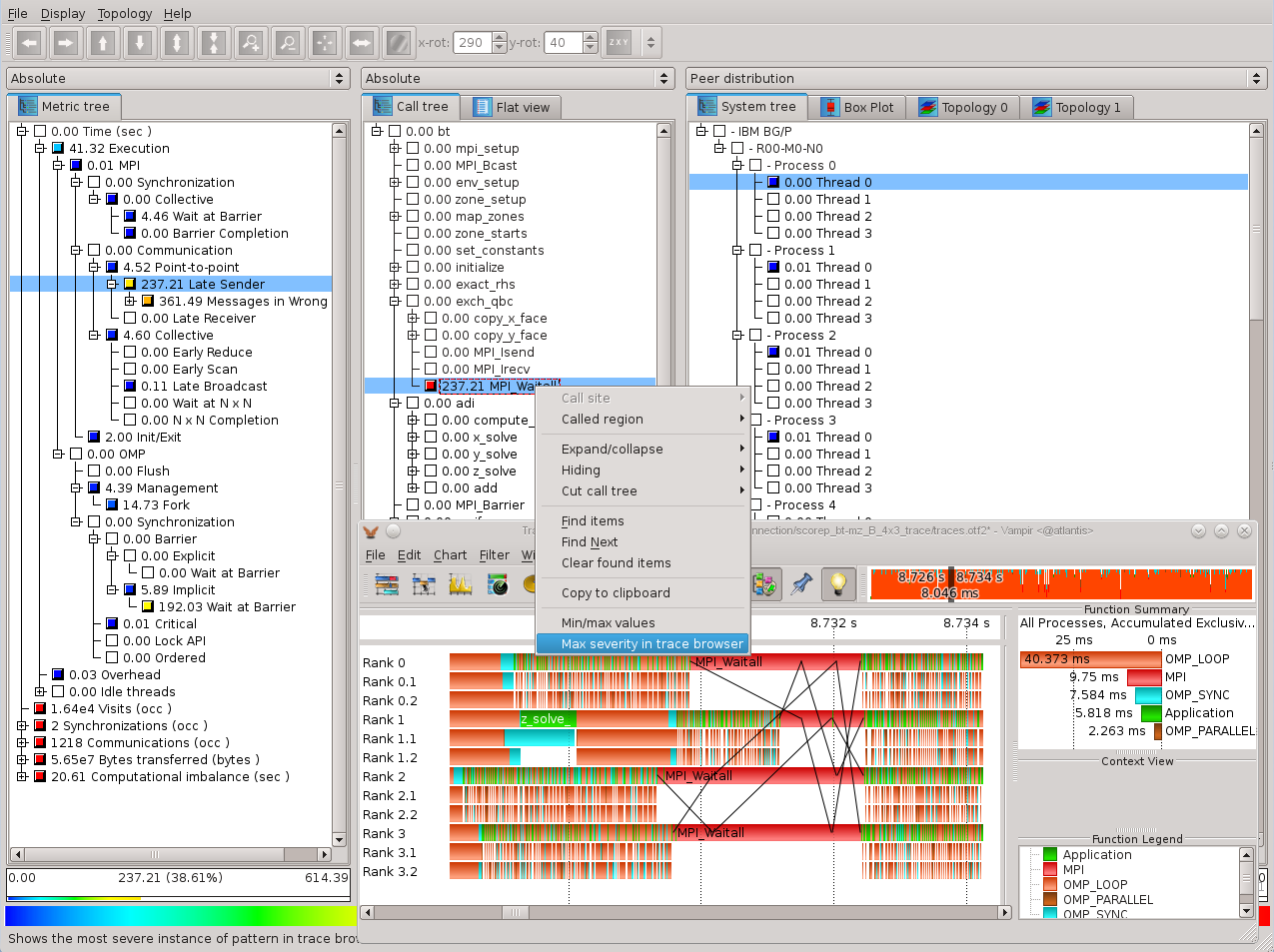
Context menu called on a special call path showing the Max severity in trace browser'' menu item which results in the location of the worst Late Broadcast instance shown in the timeline display of Vampir. It can be seen that processes enter the {{MPI}} operation earlier than the root process leading to a wait state.

Keyboard and mouse control

General control

Shift+F1	Help: What's this?
Ctrl+O	Shortcut for menu `File Open`
Ctrl+W	Shortcut for menu `File Close`
Ctrl+Q	Shortcut for menu `File Quit`
<left-mouse click>	over menu/tool bar: activate menu/function over value mode combo: select value mode over tab: switch to tab in tree: select/deselect/expand/collapse items in topology: select item
<right-mouse click>	in tree: context menu in topology: context information
Ctrl+<left-mouse click>	in tree: multiple selection/deselection
<left-mouse drag>	over scroll bar: scroll in topology: rotate topology
Ctrl+<left-mouse drag>	in topology: increase plane distance
Shift+<left-mouse drag>	in topology: move topology
<scroll mouse-wheel>="">	in topology: zoom in/out
Up arrow	in tree: move selection one item up (single-selection only) in topology/scroll area: scroll one unit up
Down arrow	in tree: move selection one item down (single-selection only) in topology/scroll area: scroll one unit down
Left arrow	in scroll area: scroll to the left
Right arrow	in scroll area: scroll to the right
Page up	in tree/topology/scroll area: scroll one page up
Page down	in tree/topology/scroll area: scroll one page down

Source code editor

Control in read only mode:

Up Arrow	Move one line up
Down Arrow	Move one line down
Left Arrow	Scroll one character to the left (if horizontally scrollable)
Right Arrow	Scroll one character to the right (if horizontally scrollable)
Page Up	Move one (viewport) page up
PageDown	Move one (viewport) page down
Home	Move to the beginning of the text
End	Move to the end of the text
<scroll mouse-wheel>="">	Scroll the page vertically
Alt+<scroll mouse-wheel>="">	Scroll the page horizontally (if horizontally scrollable)
Ctrl+<scroll mouse-wheel>="">	Zoom the text
Ctrl+A	Select all text

Additionally for the read and write mode:

Left Arrow	Move one character to the left
Right Arrow	Move one character to the right
Backspace	Delete the character to the left of the cursor
Delete	Delete the character to the right of the cursor
Ctrl+C	Copy the selected text to the clipboard
Ctrl+Insert	Copy the selected text to the clipboard
Ctrl+K	Delete to the end of the line
Ctrl+V	Paste the clipboard text into text edit
Shift+Insert	Paste the clipboard text into text edit
Ctrl+X	Delete the selected text and copy it to the clipboard
Shift+Delete	Delete the selected text and copy it to the clipboard
Ctrl+Z	Undo the last operation
Ctrl+Y	Redo the last operation
Ctrl+Left arrow	Move the cursor one word to the left
Ctrl+Right arrow	Move the cursor one word to the right
Ctrl+Home	Move the cursor to the beginning of the text
Ctrl+End	Move the cursor to the end of the text
Hold Shift + some movement (e.g., Right arrow)	Select region

Performance Algebra and Tools

As performance tuning of parallel applications usually involves multiple experiments to compare the effects of certain optimization strategies, CUBE offers a mechanism called performance algebra that can be used to merge, subtract, and average the data from different experiments and view the results in the form of a single ``derived'' experiment. Using the same representation for derived experiments and original experiments provides access to the derived behavior based on familiar metaphors and tools in addition to an arbitrary and easy composition of operations. The algebra is an ideal tool to verify and locate performance improvements and degradations likewise. The algebra includes three operators—diff, merge, and mean—provided as command-line utilities which take two or more CUBE files as input and generate another CUBE file as output. The operations are closed in the sense that the operators can be applied to the results of previous operations. Note that although all operators are defined for any valid CUBE data sets, not all possible operations make actually sense. For example, whereas it can be very helpful to compare two versions of the same code, computing the difference between entirely different programs is unlikely to yield any useful results.

Difference

Changing a program can alter its performance behavior. Altering the performance behavior means that different results are achieved for different metrics. Some might increase while others might decrease. Some might rise in certain parts of the program only, while they drop off in other parts. Finding the reason for a gain or loss in overall performance often requires considering the performance change as a multidimensional structure. With CUBE's difference operator, a user can view this structure by computing the difference between two experiments and rendering the derived result experiment like an original one. The difference operator takes two experiments and computes a derived experiment whose severity function reflects the difference between the minuend's severity and the subtrahend's severity.

The possible output is presented below.

user@host: cube_diff scout.cube remapped.cube -o result.cube
Reading scout.cube ... done.
Reading remapped.cube ... done.
++++++++++++ Diff operation begins ++++++++++++++++++++++++++
INFO::Merging metric dimension... done.
INFO::Merging program dimension... done.
INFO::Merging system dimension... done.
INFO::Mapping severities... done.
INFO::Adding topologies...
        Topology retained in experiment.
 done.
INFO::Diff operation... done.
++++++++++++ Diff operation ends successfully ++++++++++++++++
Writing result.cube ... done.

Usage:: cube_diff [-o output] [-c] [-C] [-h] minuend subtrahend
-o: Name of the output file (default: diff.cube)
-c: Do not collapse system dimension, if experiments are incompatible
-C: Collapse system dimension
-h: Help; Output a brief help message.

Merge

The merge operator's purpose is the integration of performance data from different sources. Often a certain combination of performance metrics cannot be measured during a single run. For example, certain combinations of hardware events cannot be counted simultaneously due to hardware resource limits. Or the combination of performance metrics requires using different monitoring tools that cannot be deployed during the same run. The merge operator takes an arbitrary number of CUBE experiments with a different or overlapping set of metrics and yields a derived CUBE experiment with a joint set of metrics.

The possible output is presented below.

user@host: cube_merge scout.cube remapped.cube -o result.cube
++++++++++++ Merge operation begins ++++++++++++++++++++++++++
Reading scout.cube ... done.
Reading remapped.cube ... done.
INFO::Merging metric dimension... done.
INFO::Merging program dimension... done.
INFO::Merging system dimension... done.
INFO::Mapping severities... done.
INFO::Merge operation...
        Topology retained in experiment.

        Topology retained in experiment.
 done.
++++++++++++ Merge operation ends successfully ++++++++++++++++
Writing result.cube ... done.

Usage:: cube_merge [-o output] [-c] [-C] [-h] cube ...
-o: Name of the output file (default: merge.cube)
-c: Do not collapse system dimension, if experiments are incompatible
-C: Collapse system dimension
-h: Help; Output a brief help message.

Mean

The mean operator is intended to smooth the effects of random errors introduced by unrelated system activity during an experiment or to summarize across a range of execution parameters. You can conduct several experiments and create a single average experiment from the whole series. The mean operator takes an arbitrary number of arguments.

The possible output is presented below.

user@host: cube_mean scout1.cube scout2.cube scout3.cube scout4.cube -o mean.cube
++++++++++++ Mean operation begins ++++++++++++++++++++++++++
Reading scout1.cube ... done.
INFO::Merging metric dimension... done.
INFO::Merging program dimension... done.
INFO::Merging system dimension... done.
INFO::Mapping severities... done.
INFO::Adding topologies... done.
INFO::Mean operation... done.
Reading scout2.cube ... done.
INFO::Merging metric dimension... done.
INFO::Merging program dimension... done.
INFO::Merging system dimension... done.
INFO::Mapping severities... done.
INFO::Adding topologies... done.
INFO::Mean operation... done.
Reading scout3.cube ... done.
INFO::Merging metric dimension... done.
INFO::Merging program dimension... done.
INFO::Merging system dimension... done.
INFO::Mapping severities... done.
INFO::Adding topologies... done.
INFO::Mean operation... done.
Reading scout4.cube ... done.
INFO::Merging metric dimension... done.
INFO::Merging program dimension... done.
INFO::Merging system dimension... done.
INFO::Mapping severities... done.
INFO::Adding topologies... done.
INFO::Mean operation... done.
++++++++++++ Mean operation ends successfully ++++++++++++++++
Writing mean.cube ... done.

Usage:: cube_mean [-o output] [-c] [-C] [-h cube ...
-o: Name of the output file (default: mean.cube)
-c: Do not collapse system dimension, if experiments are incompatible
-C: Collapse system dimension
-h: Help; Output a brief help message.

Compare

Compares two experiments and prints out if they are equal or not. Two experiments are equal if they have same dimensions hierarchy and the equal values of the severieties.

An example of the output is below.

user@host: cube_cmp remapped.cube scout1.cube
Reading remapped.cube ... done.
Reading scout1.cube ... done.
++++++++++++ Compare operation begins ++++++++++++++++++++++++++
Experiments are not equal.
+++++++++++++ Compare operation ends successfully ++++++++++++++++

Usage:: cube_cmp [-h] cube1 cube2
-h: Help; Output a brief help message.

Clean

CUBE files may contain more data in the definition part than absolutely necessary. The cube_clean utility creates a new CUBE file with an identical structure as the input experiment, but with the definition part cleaned up.

An example of the output is presented below.

user@host: cube_clean remapped.cube -o cleaned.cube
++++++++++++ Clean operation begins ++++++++++++++++++++++++++
Reading remapped.cube ... done.

        Topology retained in experiment.
++++++++++++ Clean operation ends successfully ++++++++++++++++
Writing cleaned.cube ... done.

Usage:: cube_clean [-o output] [-h cube
-o: Name of the output file (default: clean.cube|.gz)
-h: Help; Output a brief help message.

Reroot, Prune

For the detailed study of some part of the execution, the CUBE file can be modified based on a given call-tree node. Two different operations are possible:

The call tree may be re-rooted, i.e., only sub-trees with the given call-tree node as root are retained in the experiment.
An entire sub-tree may be pruned, i.e., removed from the experiment. In this case, all metric values for that sub-tree will be attributed to it's parent call-tree node (= ``inlined'').

An example of the output is presented below.

user@host: cube_cut -r inner_auto_ -p flux_err_ -o cutted.cube remapped.cube
Reading remapped.cube ... done.
++++++++++++ Cut operation begins ++++++++++++++++++++++++++

        Topology retained in experiment.
++++++++++++ Cut operation ends successfully ++++++++++++++++
Writing cutted.cube ... done.

Usage:: cube_cut [-h] [-r nodename] [-p nodename] [-o output cube
-o: Name of the output file (default: cut.cube|.gz)
-r: Re-root call tree at named node
-p: Prune call tree from named node (= ''inline'')
-h: Help; Output a brief help message.

Remap (version 2)

A more flixible implementation of the tool cube_remap is the cube_remap2.

This tool takes a remapping specification file as a command line argument and perform recalculation of the metric values according to the specified rules, expressed in CubePL syntax.

This tool can be used to convert all derived metrics into usual metrics, which are holding data (notice, that POSTDERIVED metrics became invalid while this conversion ).

CUBE provides examplees of remapping specification files for SCOUT and Score-P. They are stored in the directory [prefix]/share/doc/cube/examples

Usage:: ./cube_remap2 -r <remap specification file> [-o output] [-d] [-s] [-h] <cube experiment>
-r: Name of the remapping specification file. By omitting this option the specification file from the cube experiment is taken if present.
-c: Create output file with the same structure as an input file. It overrides option "-r"
-o: Name of the output file (default: remap)
-d: Convert all prederived metrics into usual metrics, calculate and store their values as a data.
-s: Add hardcoded SCALSCA metrics "Idle threads" and "Limited parallelizm"
-h: Help; Output a brief help message.

Statistics

Extracts statistical information from the CUBE files.

user@host: ./cube_stat  -m time,mpi -p remapped.cube -%
MetricRoutine     Count    Sum       Mean      Variance  Minimum      ...  Maximum
time INCL(MAIN__)    4  143.199101  35.799775  0.001783   35.759769   ...  35.839160
time   EXCL(MAIN__)  4    0.078037   0.019509  0.000441    0.001156   ...   0.037711
time   task_init_    4    0.568882   0.142221  0.001802    0.102174   ...   0.181852
time   read_input_   4    0.101781   0.025445  0.000622    0.000703   ...   0.051980
time   decomp_       4    0.000005   0.000001  0.000000    0.000001   ...   0.000002
time   inner_auto_   4  142.361593  35.590398  0.000609   35.566589   ...  35.612125
time   task_end_     4    0.088803   0.022201  0.000473    0.000468   ...   0.043699

mpi  INCL(MAIN__)    4   62.530811  15.632703  2.190396   13.607989   ...  17.162466
mpi    EXCL(MAIN__)  4    0.000000   0.000000  0.000000    0.000000   ...   0.000000
mpi    task_init_    4    0.304931   0.076233  0.001438    0.040472   ...   0.113223
mpi    read_input_   4    0.101017   0.025254  0.000633    0.000034   ...   0.051952
mpi    decomp_       4    0.000000   0.000000  0.000000    0.000000   ...   0.000000
pi    inner_auto_    4   62.037503  15.509376  2.194255   13.478049   ...  17.031288
mpi    task_end_     4    0.087360   0.021840  0.000473    0.000108   ...   0.043333

user@host: ./cube_stat  -t33 remapped.cube -p -m time,mpi,visits
Region        NumberOfCalls ExclusiveTime InclusiveTime      time       mpi      visits
sweep_                   48     76.438435    130.972847   76.438435   0.000000      48
MPI_Recv              39936     36.632249     36.632249   36.632249  36.632249   39936
MPI_Send              39936     17.684986     17.684986   17.684986  17.684986   39936
MPI_Allreduce           128      7.383530      7.383530    7.383530   7.383530     128
source_                  48      3.059890      3.059890    3.059890   0.000000      48
MPI_Barrier              12      0.382902      0.382902    0.382902   0.382902      12
flux_err_                48      0.380047      1.754759    0.380047   0.000000      48
TRACING                   8      0.251017      0.251017    0.251017   0.000000       8
MPI_Bcast                16      0.189381      0.189381    0.189381   0.189381      16
MPI_Init                  4      0.170402      0.419989    0.170402   0.170402       4
snd_real_             39936      0.139266     17.824251    0.139266   0.000000   39936
MPI_Finalize              4      0.087360      0.088790    0.087360   0.087360       4
initialize_               4      0.084858      0.168192    0.084858   0.000000       4
initxs_                   4      0.083242      0.083242    0.083242   0.000000       4
MAIN__                    4      0.078037    143.199101    0.078037   0.000000       4
rcv_real_             39936      0.077341     36.709590    0.077341   0.000000   39936
inner_                    4      0.034985    142.337220    0.034985   0.000000       4
inner_auto_               4      0.024373    142.361593    0.024373   0.000000       4
task_init_                4      0.014327      0.568882    0.014327   0.000000       4
read_input_               4      0.000716      0.101781    0.000716   0.000000       4
octant_                 416      0.000581      0.000581    0.000581   0.000000     416
global_real_max_         48      0.000441      1.374712    0.000441   0.000000      48
global_int_sum_          48      0.000298      5.978850    0.000298   0.000000      48
global_real_sum_         32      0.000108      0.030815    0.000108   0.000000      32
barrier_sync_            12      0.000105      0.383007    0.000105   0.000000      12
bcast_int_               12      0.000068      0.189395    0.000068   0.000000      12
timers                    2      0.000044      0.000044    0.000044   0.000000       2
initgeom_                 4      0.000042      0.000042    0.000042   0.000000       4
initsnc_                  4      0.000038      0.000050    0.000038   0.000000       4
task_end_                 4      0.000013      0.088803    0.000013   0.000000       4
bcast_real_               4      0.000010      0.000065    0.000010   0.000000       4
decomp_                   4      0.000005      0.000005    0.000005   0.000000       4
timers_                   2      0.000004      0.000048    0.000004   0.000000       2

Usage:

cube_stat [-h] [-p] [-m metric[,metric...] -%] [-r routine[,routine...] cubefile

OR

cube_stat -h] [-p] [-m metric[,metric...] -t topN cubefile

-h

Display this help message

-p

Pretty-print statistics (instead of CSV output)

-%

Provide statistics about process/thread metric values

-m

List of metrics (default: time)

-r

List of routines (default: main)

-t

Number for topN regions flat profile

from TAU to CUBE

Converts a profile generated by the TAU Performance System into the CUBE format. Currently, only 1-level, 2-level and full call-path profiles are supported.

An example of the output is presented below.

user@host: ./tau2cube3 tau2 -o b.cube
    Parsing TAU profile...
    tau2/profile.0.0.2
    tau2/profile.1.0.0
    Parsing TAU profile...          done.
    Creating CUBE profile...
    Number of call paths : 5
    Childmain int (int, char **)
    Number of call paths : 5
    ChildsomeA void (void)
    Number of call paths : 5
    ChildsomeB void (void)
    Number of call paths : 5
    ChildsomeC void (void)
    Number of call paths : 5
    ChildsomeD void (void)
    Path to Parents : 5
    Path to Child : 1
    Number of roots : 5
    Call-tree node created
    Call-tree node created
    Call-tree node created
    Call-tree node created
    Call-tree node created
    value time :: 8.0151
    value ncalls :: 1
    value time :: 11.0138
    value ncalls :: 1
    value time :: 8.01506
    value ncalls :: 1
    value time :: 11.0138
    value ncalls :: 1
    value time :: 5.00815
    value ncalls :: 1
    value time :: 11.0138
    value ncalls :: 1
    value time :: 0.000287
    value ncalls :: 1
    value time :: 11.0138
    value ncalls :: 1
    value time :: 0
    value ncalls :: 0
    value time :: 9.00879
    value ncalls :: 1
    done.

Usage:: tau2cube [tau-profile-dir ][-o cube]

Common Calltree

Common Calltree is a tool to reduce call trees of a set of cube files to the common part.

Usage:: cube_commoncalltree cubefile1 cubefile2 ... cubefileN

The tool cube_commoncalltree takes set of input cubefiles

(cubefile1 cubefile2 ... cubefileN)

and creates corresponding set of cube files

(cubefile1_commoncalltree cubefile2_commoncalltree ... cubefileN_commoncalltree).

Output cube files cubefileX_commoncalltree do have the equal system and metric dimensions like corresponding cubefileX file.

Call trees among cubefileX_commoncalltree files are reduced to the maximal (up to a special case in region naming scheme) common part. Inclusive value of the "missing" part is added as a exclusive value to its parent (which is a part of common part of call tree)

This tool is particulary useful for comparison of exprerimens with the different recursion depth or with the additional sub call trees depending on some loop iteration index.

Topology Assistant

Topology assistant is a tool to handle topologies in cube files. It is able to add or edit a topology.

Usage:: cube_topoassist {OPTION} cubefile

The current available options are:

To create a new topology in an existing cube file,
To [re]name an existing virtual topology, and
To [re]name the dimensions of a virtual topology.

The command-line switches for this utility are:

-c: creates a new topology in a given cube file.

-n: displays a numbered list of the existing topologies in the given cube file, and lets the user choose one to be named or renamed.

-d: displays the existing topologies, and lets the user name the dimensions of one of them.

The resulting CUBE file is named topo.cube[.gz], in the current directory.

As mentioned abot, when using the -d or -n command-line options, a numbered list of the current topologies will appear, showing the topology names, its dimension names (when existing), and the number of coordinates in each dimension, as well as the total number of threads. This is an example of the usage:

$ cube_topoassist topo.cube.gz -n
Reading topo.cube.gz . Please wait... Done.
Processes are ordered by rank. For more information about this file, 
use cube_info -S <cube experiment>

This CUBE has 3 topologie(s).
0. <Unnamed topology>, 3 dimensions: x: 3, y: 1, z: 4. Total = 12 threads. 
1. Test topology, 1 dimensions: dim_x: 12. Total = 12 threads. 
2. <Unnamed topology>, 3 dimensions: 3, 1, 4. Total = 12 threads. <Dimensions are not named>


Topology to [re]name?
1 
New name: 
Hardware topology
Topology successfully [re]named.

Writing topo.cube.gz ... done.

The process is similar for [re]naming dimensions within a topology. One characteristic is that either all dimensions are named, or none.

One could easily create a script to generate the coordinates according to some algorithm/equation, and feed this to the assistant as an input. The only requirement is to answer the questions in the order they appear, and after that, feed the coordinates. Coordinates are asked for in rank order, and inside every rank, in thread order.

The sequence of questions made by the assistant when creating a new topology (the -c switch) is:

New topology's name
Number of dimensions
Will the above dimensions be named? (Y/N)
If yes, asks the name. Empty is not valid.
Number of coordinates in that dimension
Asks if this dimension is either periodic or not (Y/N)
Repeat the previous three steps for every dimension
After that, it expects the coordinates for each thread in this topology, separated by spaces, in the order described above.

This is a sample session of the assistant:

$ cube_topoassist -c experiment.cube.gz
Reading experiment.cube.gz. Please wait... Done.
Processes are ordered by rank. For more information about this file, use cube_info -S <cube experiment>

So far, only cartesian topologies are accepted.
Name for new topology?
Test topology
Number of Dimensions?
3
Do you want to name the dimensions (axis) of this topology? (Y/N)
y
Name for dimension 0
torque
Number of elements for dimension 0
2000
Is dimension 0 periodic?
y
Name for dimension 1
rotation
Number of elements for dimension 1
1500
Is dimension 1 periodic?
n
Name for dimension 2
period
Number of elements for dimension 2
50
Is dimension 2 periodic?
n
Alert: The number of possible coordinates (150000000) is bigger than the number of threads
 on the specified cube file (12). Some positions will stay empty.
Topology on THREAD level.
Thread 0's (rank 0) coordinates in 3 dimensions, separated by spaces
0 0 0
0 0 1
0 0 2
...
...
...
Writing topo.cube.gz ... done.
$

So, a possible input file for this cube experiment could be:

Test topology
3
y
torque
2000
y
rotation
1500
n
period
50
n
0 0 0
0 0 1
0 0 2
... (the remaining coordinates)

And then call the assistant:: cube_topoassist -c cubefile.cube < input.txt

Dump

To export values from the cube report into another tool or to examine internal structure of the cube report CUBE framework provedes a tool cube_dump tool, which prints out different values. It calculates inclusive and exclusive values along metric tree and call tree, agregates over system tree or displays values for every thread separately. In addition it provides user to define new metrics(see file CubeDerivedMetrics.pdf). Results are calculated and shown. For convenience user can invoke defined metrics along with new once in any order. For doing so one lists unique names of metrics separated by commas. For access to more than one callpaths, user can specify the ids or a range of them like "2-9". This also can be done for threads. Additionally provides a calculation of the flat profile values.

-m <metrics>|<new metrics>|all|<filename>: Select one or more of metrics (unique names) for data dump.
: By giving a CubePL expression one can define one or more new metrics by giving correspond formula. If the expression prefixed with "\<name\>:", <name> is used as a unique name for the new metric.
: <filename> - takes a CubePL expression from file <filename> and defines a derived metric with it
: all - all metrics will be printed.
: Combination of these three is possible.
-c <cnode ids>|all|leafs|roots|level>X|level=X|level<X|name=/regexp/|<filename>
: Select one or more call paths to be printed out .
: <cnode ids> - list or range of call path ids: 0,3,5-10,25
: all - all call paths are printed
: leafs - only call paths without children are printed
: roots - only root cnodes are printed
: level<X, level=X or level>X - only cnodes of the level more, equal or less than N are printed
: name=/regexp/- only cnodes with the region name matching to the regular expression regexp
: <filename> - takes a CubePL expression from file <filename> and evaluates it for every callpath.
: If the result is non-zero - call path is included into the output.
-x incl|excl: Selects, if the data along the metric tree should be calculated as an inclusive or an exclusive value.
: (Default value: incl).
-z incl|excl|stored: Selects, if the data along the call tree should be calculated as an inclusive or an exclusive value.
: (Default value: excl).
-t <thread id>|aggr: Show data for one or more selected threads or aggregated over system tree.
-r: Prints aggregated values for every region (flat profile), sorted by id.
-f <name>: Selects a stored data with the name <name> to display
-d: Shows the coordinates for every topology as well.
-y: Disables expansion of clusters and shows bare stored meta structure.
-w: Prints out the information about structure of the cube.
-o <filename>|-: Uses a device or STDOUT for the output. If omit, STDOUT is used.
-s human|gnuplot|gnuplot2|csv|csv2|R: Uses either human readable form, GNUPLOT or CSV (two different layouts) format or binary R matrix for data export.
-h|-?: Help; Output a brief help message.

This is examples of the usage.

Example 1:

$cube_dump -m time,"metric::visits(e)","metric::time(i)/metric::visits(e)" -c 0 \
  -z incl -s gnuplot  profile.cubex 

# ===================== DATA =================== 
# Print out the data of the metric time
#main(id=0)
0   0   80.549003343
0   1   44.115097986
0   2   43.486614165
0   3   43.940738098
0   4   80.539393011
0   5   42.723353088
0   6   42.61159706
0   7   43.108220977
0   8   80.635220741
0   9   43.788284208
0   10  43.831524441
0   11  43.652044759
0   12  80.629776666
0   13  42.692885677
0   14  42.719330066
0   15  42.732487708

# Print out the data of the metric New Metric1
#main(id=0)
0   0   80.549003343
0   1   1.79769313486e+308
0   2   1.79769313486e+308
0   3   1.79769313486e+308
0   4   80.539393011
0   5   1.79769313486e+308
0   6   1.79769313486e+308
0   7   1.79769313486e+308
0   8   80.635220741
0   9   1.79769313486e+308
0   10  1.79769313486e+308
0   11  1.79769313486e+308
0   12  80.629776666
0   13  1.79769313486e+308
0   14  1.79769313486e+308
0   15  1.79769313486e+308

# Print out the data of the metric New Metric2
#main(id=0)
0   0   1
0   1   0
0   2   0
0   3   0
0   4   1
0   5   0
0   6   0
0   7   0
0   8   1
0   9   0
0   10  0
0   11  0
0   12  1
0   13  0
0   14  0
0   15  0

Example 2:

$cube_dump -m time -s gnuplot2  profile.cubex 

# ===================== CONFIGURE GNUPLOT =================== 
set logscal x ; set logscal y ; set grid ; set xrange [16:300000] 
; set terminal png size "600,400"

# ===================== DATA =================== 
# Print out the data of the metric time

;set output "0.png" 
; plot 6.4e-18*x**(5.0/2.0) + 5.2e-05 t "setPrecision(int, PrecisionFormat)(id=18)" , 
1.2e-17*x**(7.0/3.0) + 3.6e-05 t "setRoundNr(int, PrecisionFormat)(id=19)" , 
2.1e-17*x**(9.0/4.0) + 3.1e-05 t "setUpperExpNr(int, PrecisionFormat)(id=20)" , 
7.1e-19*x**(5.0/2.0) + 8.8e-06 t "getInstance()(id=21)" , 
2.8e-18*x**(2.0/1.0)*log(x) + 3.3e-06 t "getCubePluginCount()(id=24)"

;set output "1.png" 
; plot 1.3e-20*x**(5.0/2.0)*log(x) + 4.2e-06 t "PluginList()(id=25)" , 
9.7e-18*x**(7.0/3.0) + 1.1e-05 t "loadContextFreePlugin(PluginData&)(id=28)" , 
1e-17*x**(9.0/4.0) + 8.8e-06 t "loadCubePlugin(PluginData&)(id=29)" , 
1e-18*x**(9.0/4.0) + 1.1e-06 t "name() const(id=35)" , 
2.6e-18*x**(2.0/1.0)*log(x) + 3.7e-06 t "getCubePlugin(int)(id=44)"

Example 3:

$cube_dump -m time,"metric::visits(e)","metric::time(i)/metric::visits(e)" -c 0 \
 -t aggr  -z incl -s human  profile.cubex 

 ===================== DATA =================== 
Print out the data of the metric time

            All threads
-------------------------------------------------------------------------------
main(id=0)  841.755571994
Print out the data of the metric New Metric1

            All threads
-------------------------------------------------------------------------------
main(id=0)  210.438892999
Print out the data of the metric New Metric2

            All threads
-------------------------------------------------------------------------------
main(id=0)  4

Example 4:

$cube_dump -m time,"metric::visits(e)","metric::time(i)/metric::visits(e)" -c 20 \
  -z incl -s csv  profile.cubex 
  
20,0,8.9812e-05
20,1,0
20,2,0
20,3,0
20,4,9.7463e-05
20,5,0
20,6,0
20,7,0
20,8,0.000132327
20,9,0
20,10,0
20,11,0
20,12,7.2788e-05
20,13,0
20,14,0
20,15,0

20,0,8.9812e-05
20,1,-1.79769313486e+308
20,2,-1.79769313486e+308
20,3,-1.79769313486e+308
20,4,9.7463e-05
20,5,-1.79769313486e+308
20,6,-1.79769313486e+308
20,7,-1.79769313486e+308
20,8,0.000132327
20,9,-1.79769313486e+308
20,10,-1.79769313486e+308
20,11,-1.79769313486e+308
20,12,7.2788e-05
20,13,-1.79769313486e+308
20,14,-1.79769313486e+308
20,15,-1.79769313486e+308

20,0,1
20,1,0
20,2,0
20,3,0
20,4,1
20,5,0
20,6,0
20,7,0
20,8,1
20,9,0
20,10,0
20,11,0
20,12,1
20,13,0
20,14,0
20,15,0

Example 5:

$cube_dump -m time,"metric::visits(e)","metric::time(i)/metric::visits(e)" -c 1 \
  -z incl -s csv2  profile.cubex 
  
Cnode ID, Thread ID,time,New Metric1,New Metric2
1,0,80.548967177,80.548967177,1
1,1,44.115097986,1.79769313486e+308,0
1,2,43.486614165,1.79769313486e+308,0
1,3,43.940738098,1.79769313486e+308,0
1,4,80.539359524,80.539359524,1
1,5,42.723353088,1.79769313486e+308,0
1,6,42.61159706,1.79769313486e+308,0
1,7,43.108220977,1.79769313486e+308,0
1,8,80.635176341,80.635176341,1
1,9,43.788284208,1.79769313486e+308,0
1,10,43.831524441,1.79769313486e+308,0
1,11,43.652044759,1.79769313486e+308,0
1,12,80.629742485,80.629742485,1
1,13,42.692885677,1.79769313486e+308,0
1,14,42.719330066,1.79769313486e+308,0
1,15,42.732487708,1.79769313486e+308,0

Example 6:

$cube_dump -m time,"metric::visits(e)","metric::time(i)/metric::visits(e)" -c 1 \
  -z incl -s R  profile.cubex -o output_file

This will generate binary file "output_file" which can be loaded in R. In consists of three matrices, each one corresponding to one metric. Each matrix is named after the metric and it contains values for all threads and nodes.

Example 7: We select only call path names, starting with "main" using the CubePL expression (stored in file name "selection.cubepl") :

{ 
${a}=0;
if (${cube::region::name}[${calculation::region::id}] =~  /^main/ )
{ ${a}=1; }; return ${a}; 
}

Then:

cube_dump -m time,"metric::visits(e)","metric::time(i)/metric::visits(e)"   -c selection.cubepl  \
 -z incl  -t aggr  profile.cubex  

 ===================== DATA =================== 
Print out the data of the metric time
                  All threads
-------------------------------------------------------------------------------
main(id=0)        841.755571994
main_loop(id=12)  840.73706946

Print out the data of the metric New Metric1
                  All threads
-------------------------------------------------------------------------------
main(id=0)        210.438892999
main_loop(id=12)  0.210184267365

Print out the data of the metric New Metric2
                  All threads
-------------------------------------------------------------------------------
main(id=0)        4
main_loop(id=12)  4000

Options "leafs", "roots", "level=", "level<", "level>" and "name=/regexp/" are shortcuts for a build-in CubePL expression, which is used to select a call path.

"leafs" : stands for:

{ 
${a}=0;
if (${cube::callpath::#children}[${calculation::callpath::id}] == 0 )
{ ${a}=1; }; return ${a}; 
}

"roots" : stands for:

{ 
${a}=0;
if (${cube::callpath::parent::id}[${calculation::callpath::id}] == -1 )
{ ${a}=1; }; return ${a}; 
}

"level=N" : stands for:

{ 
${level}=N;
${index}=0;
${i}=${calculation::callpath::id};
while (${cube::callpath::parent::id}[${i}] != -1 )
{ ${i}= ${cube::callpath::parent::id}[${i}]; ${index}=${index}+1; }; 
${a}=0;
if (${index} ==  ${level})
{${a}=1; };
return ${a}; 
}

"name=/regexp/" : stands for:

{ 
  ${a}=0;
   if ( ${cube::region::name}[${calculation::region::id}] =~  /regexp/ )
  { ${a}=1; }; return ${a}; 
};

"level<N" and "level>N" differ from "level=N" in the boolean operation in the line 8. For detailed documentation of the syntax of CubePL please see .