Helical peptides

Small helical peptides are among the easiest proteins to fold in simulations. Typically these peptides have a few turns of an α-helix and are too short to have any complex tertiary structure. The regular structure of an α-helix is a natural compact structure for poly-peptide chains. The residues making hydrogen bonds with each other are close in sequence, so that local interactions can easily lead such small peptides to fold into helices.

Normally the search for the native state for such peptides goes extremely fast in PROFASI. Often structures very close to the native structures are found within about 10-30 seconds of starting the simulations from completely random initial conformations, using nothing more than canonical Monte Carlo simulations. This is demonstrated in the first tutorial of PROFASI, using the well known Tryptophan cage peptide. To get good thermodynamic distributions using as little computing time as possible, one uses generalised ensemble techniques such as parallel tempering or simulated tempering.

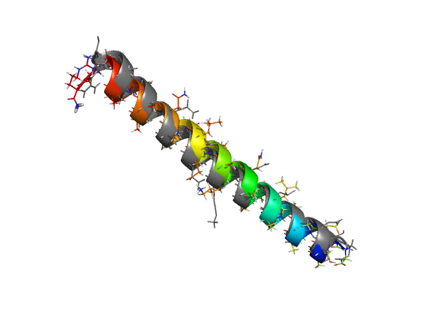
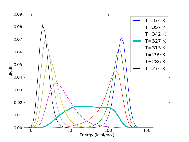
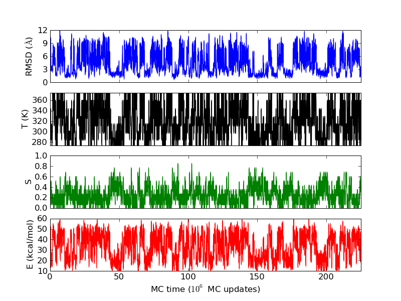
As an example, let's consider the 37 residue winter flounder antifreeze peptide HPLC-6 shown above. This is a particularly simple peptide. The plots shown here are based on data generated with a 4 hour parallel tempering simulation, using 16 processors. Each replica started with a different random initial conformation and a different random number seed. There were 8 temperatures geometrically distributed (Tn=T0· rn) between 274 K and 374 K. Let's start with traces of the run time history from the replicas. This is what one normally looks at first, to see if everything is OK with the runs. The runs had about 200 million elementary MC updates.

Run time history of the backbone RMSD for the 16 nodes used for the 4 hour test run with the HPLC-6 peptide. Each run moves back and forth between a folded state with RMSD around 2 Å and 15 Å. Each run is different, but there is nothing special about any one of them.

Left: For the HPLC-6 peptide, here are energy (E), helix content (H), temperature (T) and RMSD as functions of MC time, as seen in one of the replicas. Right: Same as the left figure, but for the fs peptide (sequence SUC-AAAAA AAARA AAARA AAARA A-NH2). The HPLC-6 system, shown in these examples has not been chosen because it is the most well behaved system I know for parallel tempering runs. It is one of the systems where looking at the data inspires faith in the orderliness of the universe, but there are other systems, like fs, where things move much faster.

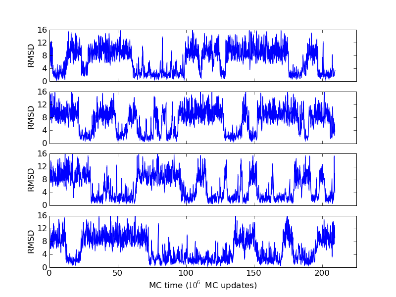
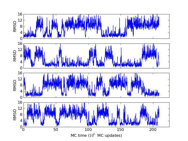
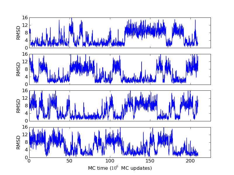
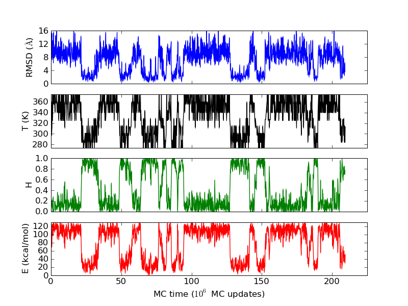
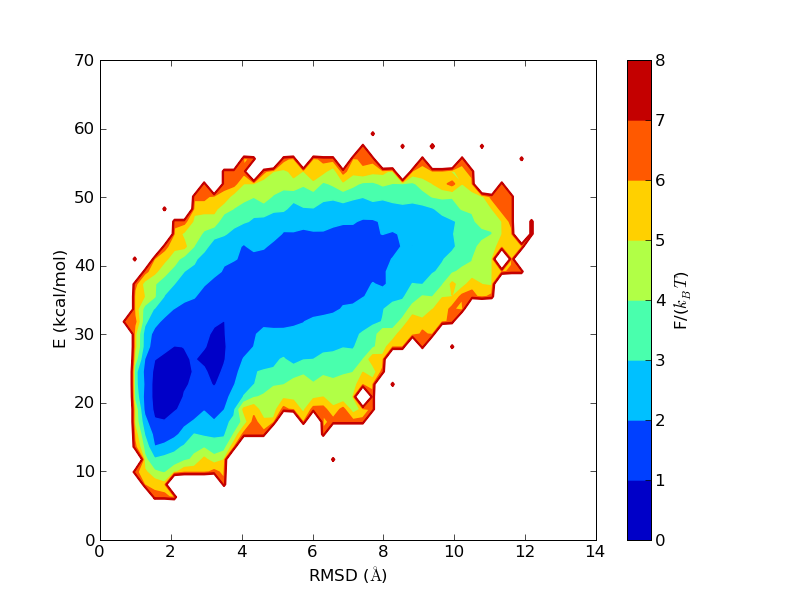
The above figures illustrate many aspects of replica exchange Monte Carlo simulations. In these plots, one gets an impression that we are dealing with a two state system. If energy is used as the only characterising feature of a protein conformation, it is indeed a two state system. The system moves back and forth between a high and a low energy state. The low energy state corresponds to high helix content and low RMSD values. Small RMSD values like 2 Å for a 37 residue peptide identify a fairly unique conformation. It is very likely that our low energy state above corresponds to a set of structures in which all members are conformationally similar to all others. Large RMSD values don't identify a structure uniquely. If two structures are both 15 Å in RMSD from a reference structure, it is like saying that you and me both look very different from George Bush. This does not mean that we have anything in common. The high energy conformations seen in these simulations contain conformationally diverse structures. This point is brought out more clearly in the following figure.

Left: Scatter plot of RMSD and the radius of gyration colour coded with energy. We see that the high energy high RMSD structures have a wide spread in the radius of gyration, showing that the high energy state is conformationally inhomogeneous. This figure also shows why some people like to talk about a folding "funnel". Right: Energy histogram at different temperatures.

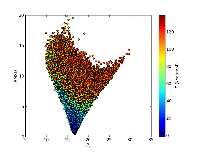
The funnel like energy landscape of this protein seen in the above figure explains why the simulations are so well behaved. Let's remember that these simulations are done with an all-atom, sequence based force field, which uses no information on the experimentally determined structure. That the lowest energy state has such a low RMSD is an output of the simulation, not its input.

The energy histograms shown above illustrate another interesting aspect. Even for systems which look so two state like, very seldom is there ever a temperature at which the observed temperature histogram is bimodal. What we see in the figure above is more typical. The histograms at the high and low temperature ends have hardly any overlap. The histograms in the intermediate temperatures are wider. Sometimes, like in the figure above, there is a temperature at which the energy histogram has a flat plateau, leading to a rather large variance.

β-hairpins and 3-stranded β-sheets

Left: C-terminal hairpin of protein G: (PDB id: 1GB1, residues 41-56, Sequence : GEWTYDDATKTFTVTE) Right: A designed 3 stranded β-sheet. Sequence : TWIQN GSTKW YQNGS TKIYT

β-hairpins are somewhat more complex structures than α-helices. Different regions of the chain along the sequence have different local environments, unlike helices which have an approximate translational symmetry along the helix axis. Residues making hydrogen bonds in a β-hairpin have different sequence separations, and on the average, are further apart than such residues in an α-helix. For small β-hairpins and 3-stranded β-sheet systems, the Monte Carlo search of the conformation space is nevertheless very fast. Folding as well as thermodynamic properties can be investigated using ProFASi using about the same computing time as for small helices.

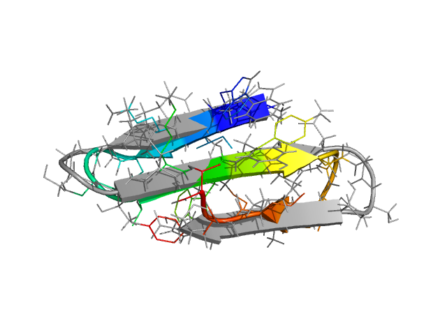
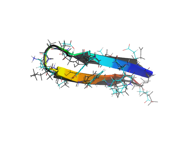
The only thing one needs to change, to go from the HPLC-6 simulation described in detail above to, for instance, the C-terminal hairpin of protein G, is the amino acid sequence. ProFASi implements a sequence based model. It does not need to know that what we are studying is "supposed to be" a β-hairpin or a helix. That should come out automatically. The only place where we need the experimentally determined structure is when we want to evaluate the simulations, and parametrise the explored conformations using RMSD with respect to the PDB structure.

In the figure above, the C-terminal hairpin (residues 41 through 56) of protein G (PDB id: 1GB1) is shown superimposed on the free energy minimum in the simulations. Two mutants of this peptide with sequences GEWTYNPATGKFTVTE and KKWTYNPATGKFTVQE have also been studied with the model. The mutants were designed and experimentally observed to be significantly more stable than the wild type. ProFASi reproduces, the native population of the three variants of the sequence. Several other small β-sheet peptides, either hairpins or 3-stranded β-sheets, have also been studied with ProFASi.

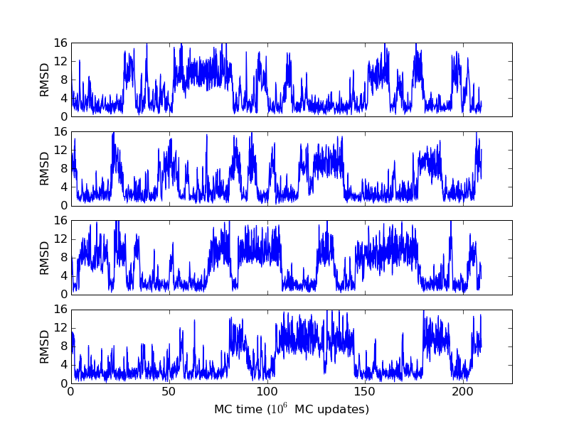
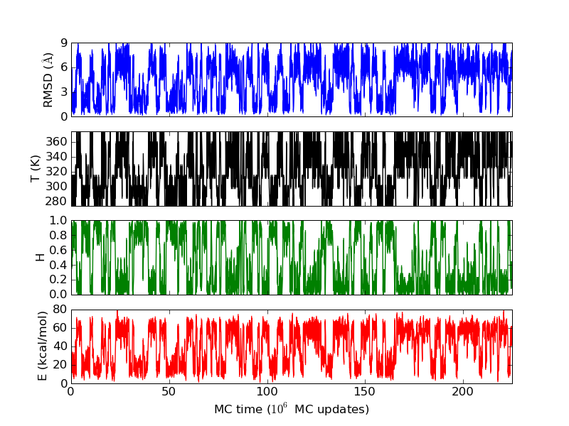
The energy and free energy landscapes seen for β-sheet peptides are somewhat more complicated than the extremely simple picture we got above for the HPLC-6 peptide. The following figures refer to a small designed β-hairpin, MBH12 with PDB id 1J4M.

Left: Run time history of energy (E), β-strand content (S), temperature and RMSD for one replica of a parallel tempering simulation of the peptide MBH12( PDB id: 1J4M, Sequence : RGKWTYNGITYEGR, 14 residues). To keep things uniform in this page, the run time history was kept to about 200 Million MC updates like for HPLC-6, which takes about 1 hour for this peptide. Right: Free energy plotted against RMSD and Energy for MBH12 at 313 K.

The run time history above superficially resembles those seen above for the helical peptides. But notice that the β-strand content does not reach 1 as the helix content did before. To make a hairpin, one needs two β-strands and a turn. The residues in the turn region are not in the β region of the Ramachandran space. The first and the last residues are not included in evaluating the secondary structure contents, as not both the Ramachandran angles are well determined in these residues. Therefore, out of 14 residues in MBH12, 12 are included in the evaluation of S, and 4 of them are in the turn. This explains why this "β-sheet" peptide does not have S close to 1 in the states with the lowest RMSD values.

β-sheet peptides often feature deep local minima, corresponding to strands attached off-register, or with the wrong set of hydrogen bonds. This is not much of a problem for MBH12, though a secondary minimum can be seen in the free energy plot above. The lower energy of the native minimum means that the secondary minimum at around 4 Å will be relatively less populated at lower temperatures.

What does an MC evolution "look" like ?

In a Markov chain Monte Carlo simulation, there is no inbuilt concept of physical time. The "Monte Carlo time" (MC time) in the plots shown in these pages is simply the number of Monte Carlo updates made on the system. A small change in one angle and a large change in the same angle might take the same (1 unit of) "MC time" if the MC move set allows both updates. For an accepted MC move, interpolation between the initial and the final state need not generate sensible intermediates. An elementary MC update is therefore unlike a small classical time interval.

Given a starting conformation of a protein chain, the set of states that can be reached with one MC update depends on the MC move set. For simulations of single protein chains, ProFASi uses the following move set:

• Random update of a randomly chosen side chain angle
• Random update of a randomly chosen backbone angle
• Concerted change of up to 8 contiguous backbone angles to make small changes to a section of the backbone, while leaving the region outside largely unaffected.

An extended protein conformation might become completely unrecognisable after a few MC updates with this set of moves. But for compact protein conformations, this is not true. A compact arrangement of a protein chain requires all its degrees of freedom to be arranged in a precise way with a small tolerance. Any degree of freedom changed beyond this tolerance causes a large change in energy, for instance, by causing the chain to intersect itself. A large random change to any degree of freedom, especially to a backbone degree of freedom, is overwhelmingly likely to be rejected. The system therefore can only reach other states in its immediate conformational neighbourhood in one MC update. The resulting slower diffusion through the conformation space is guided by the energy of the system. This gives the impression of a physical temporal evolution in Monte Carlo simulations done with ProFASi. Here is one example...

The "videos" of folding simulations you will find in the ProFASi gallery are all of this kind. They are Markov chain Monte Carlo simulations. The time variable can not be calibrated to mean an interval of physical time. They approximate diffusive motion in a potential energy landscape. They are of great value in understanding what is happening to the proteins in a simulation, and can aid hypothesis generation, since many scientists like working with mental pictures of the systems they are studying. Any qualitative picture so derived, should always be backed up with other arguments.

References

The results discussed in this page have been published in the following articles.- An Effective All Atom Potential for Proteins, Anders Irbäck, Simon Mitternacht and Sandipan Mohanty, (2009) PMC Biophysics 2:2
- Folding of proteins with diverse folds, Sandipan Mohanty and Ulrich H.E. Hansmann, (2006) Biophys. J. 91 3573
- Folding Thermodynamics of peptides, Anders Irbäck and Sandipan Mohanty (2005) Biophys. J. 88 1560