Total time spent for program execution including the idle times of CPUs
reserved for slave threads during OpenMP sequential execution. This
pattern assumes that every thread of a process allocated a separate CPU
during the entire runtime of the process.
Unit:
Seconds
Diagnosis:
Expand the metric tree hierarchy to break down total time into
constituent parts which will help determine how much of it is due to
local/serial computation versus MPI and/or OpenMP parallelization
costs, and how much of that time is wasted waiting for other processes
or threads due to ineffective load balance or due to insufficient
parallelism.
Expand the call tree to identify important callpaths and routines where
most time is spent, and examine the times for each process or thread to
locate load imbalance.
Number of times a call path has been visited. Visit counts for MPI
routine call paths directly relate to the number of MPI Communications and
Synchronizations. Visit counts for OpenMP operations and parallel regions
(loops) directly relate to the number of times they were executed.
Routines which were not instrumented, or were filtered during
measurement, do not appear on recorded call paths. Similarly, routines
are not shown if the compiler optimizer successfully in-lined them
prior to automatic instrumentation.
Unit:
Counts
Diagnosis:
Call paths that are frequently visited (and thereby have high exclusive
Visit counts) can be expected to have an important role in application
execution performance (e.g., Execution Time). Very frequently executed
routines, which are relatively short and quick to execute, may have an
adverse impact on measurement quality. This can be due to
instrumentation preventing in-lining and other compiler optimizations
and/or overheads associated with measurement such as reading timers and
hardware counters on routine entry and exit. When such routines consist
solely of local/sequential computation (i.e., neither communication nor
synchronization), they should be eliminated to improve the quality of
the parallel measurement and analysis. One approach is to specify the
names of such routines in a filter file for subsequent
measurements to ignore, and thereby considerably reduce their
measurement impact. Alternatively, selective instrumentation
can be employed to entirely avoid instrumenting such routines and
thereby remove all measurement impact. In both cases, uninstrumented
and filtered routines will not appear in the measurement and analysis,
much as if they had been "in-lined" into their calling routine.
Time spent on program execution but without the idle times of slave
threads during OpenMP sequential execution.
Unit:
Seconds
Diagnosis:
Expand the call tree to determine important callpaths and routines
where most exclusive execution time is spent, and examine the time for
each process or thread on those callpaths looking for significant
variations which might indicate the origin of load imbalance.
Where exclusive execution time on each process/thread is unexpectedly
slow, profiling with PAPI preset or platform-specific hardware counters
may help to understand the origin. Serial program profiling tools
(e.g., gprof) may also be helpful. Generally, compiler optimization
flags and optimized libraries should be investigated to improve serial
performance, and where necessary alternative algorithms employed.
Time spent performing major tasks related to measurement, such as
creation of the experiment archive directory, clock synchronization or
dumping trace buffer contents to a file. Note that normal per-event
overheads – such as event acquisition, reading timers and
hardware counters, runtime call-path summarization and storage in trace
buffers – is not included.
Unit:
Seconds
Diagnosis:
Significant measurement overheads are typically incurred when
measurement is initialized (e.g., in the program main routine
or MPI_Init) and finalized (e.g., in MPI_Finalize),
and are generally unavoidable. While they extend the total (wallclock)
time for measurement, when they occur before parallel execution starts
or after it completes, the quality of measurement of the parallel
execution is not degraded. Trace file writing overhead time can be
kept to a minimum by specifying an efficient parallel filesystem (when
provided) for the experiment archive (e.g.,
EPK_GDIR=/work/mydir) and not specifying a different
location for intermediate files (i.e., EPK_LDIR=$EPK_GDIR).
When measurement overhead is reported for other call paths, especially
during parallel execution, measurement perturbation is considerable and
interpretation of the resulting analysis much more difficult. A common
cause of measurement overhead during parallel execution is the flushing
of full trace buffers to disk: warnings issued by the EPIK measurement
system indicate when this occurs. When flushing occurs simultaneously
for all processes and threads, the associated perturbation is
localized. More usually, buffer filling and flushing occurs
independently at different times on each process/thread and the
resulting perturbation is extremely disruptive, often forming a
catastrophic chain reaction. It is highly advisable to avoid
intermediate trace flushes by appropriate instrumentation and
measurement configuration, such as specifying a filter file
listing purely computational routines (classified as type USR by
cube3_score -r ) or an adequate trace buffer size
(ELG_BUFFER_SIZE larger than max_tbc reported by
cube3_score). If the maximum trace buffer capacity requirement
remains too large for a full-size measurement, it may be necessary to
configure the subject application with a smaller problem size or to
perform fewer iterations/timesteps to shorten the measurement (and
thereby reduce the size of the trace).
This pattern refers to the time spent in (instrumented) MPI calls.
Unit:
Seconds
Diagnosis:
Expand the metric tree to determine which classes of MPI operation
contribute the most time. Typically the remaining (exclusive) MPI Time,
corresponding to instrumented MPI routines that are not in one of the
child classes, will be negligible. There can, however, be significant
time in collective operations such as MPI_Comm_create,
MPI_Comm_free and MPI_Cart_create that are considered
neither explicit synchronization nor communication, but result in
implicit barrier synchronization of participating processes. Avoidable
waiting time for these operations will be reduced if all processes
execute them simultaneously. If these are repeated operations, e.g., in
a loop, it is worth investigating whether their frequency can be
reduced by re-use.
This pattern refers to the time spent in MPI explicit synchronization
calls, i.e., barriers. Time in point-to-point messages with no data
used for coordination is currently part of MPI Point-to-point Communication Time.
Unit:
Seconds
Diagnosis:
Expand the metric tree further to determine the proportion of time in
different classes of MPI synchronization operations. Expand the
calltree to identify which callpaths are responsible for the most
synchronization time. Also examine the distribution of synchronization
time on each participating process for indication of load imbalance in
preceding code.
This pattern refers to the time spent in MPI communication calls.
Unit:
Seconds
Diagnosis:
Expand the metric tree further to determine the proportion of time in
different classes of MPI communication operations. Expand the calltree
to identify which callpaths are responsible for the most communication
time. Also examine the distribution of communication time on each
participating process for indication of communication imbalance or load
imbalance in preceding code.
This pattern refers to the time spent in MPI file I/O calls.
Unit:
Seconds
Diagnosis:
Expand the metric tree further to determine the proportion of time in
different classes of MPI file I/O operations. Expand the calltree to
identify which callpaths are responsible for the most file I/O time.
Also examine the distribution of MPI file I/O time on each process for
indication of load imbalance. Use a parallel filesystem (such as
/work) when possible, and check that appropriate hints values
have been associated with the MPI_Info object of MPI files.
Exclusive MPI file I/O time relates to individual (non-collective)
operations. When multiple processes read and write to files, MPI
collective file reads and writes can be more efficient.
This pattern refers to the time spent in collective MPI file I/O calls.
Unit:
Seconds
Diagnosis:
Expand the calltree to identify which callpaths are responsible for the
most collective file I/O time. Examine the distribution of times on
each participating process for indication of imbalance in the operation
itself or in preceding code. Examine the number of MPI File Collective Operations
done by each process as a possible origin of imbalance. Where asychrony
or imbalance prevents effective use of collective file I/O,
(non-collective) individual file I/O may be preferable.
Time spent in MPI initialization and finalization calls, i.e.,
MPI_Init or MPI_Init_thread and
MPI_Finalize.
Unit:
Seconds
Diagnosis:
These are unavoidable one-off costs for MPI parallel programs, which
can be expected to increase for larger numbers of processes. Some
applications may not use all of the processes provided (or not use some
of them for the entire execution), such that unused and wasted
processes wait in MPI_Finalize for the others to finish. If
the proportion of time in these calls is significant, it is probably
more effective to use a smaller number of processes (or a larger amount
of computation).
This pattern refers to the total time spent in MPI barriers.
Unit:
Seconds
Diagnosis:
When the time for MPI explicit barrier synchronization is significant,
expand the call tree to determine which MPI_Barrier calls are
responsible, and compare with their Visits count to see how
frequently they were executed. Barrier synchronizations which are not
necessary for correctness should be removed. It may also be appropriate
to use a communicator containing fewer processes, or a number of
point-to-point messages for coordination instead. Also examine the
distribution of time on each participating process for indication of
load imbalance in preceding code.
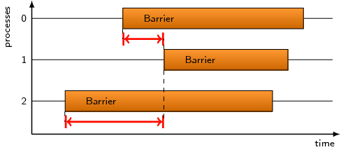
This pattern covers the time spent waiting in front of an MPI barrier,
which is the time inside the barrier call until the last processes has
reached the barrier.
Unit:
Seconds
Diagnosis:
A large amount of waiting time at barriers can be an indication of load
imbalance. Examine the waiting times for each process and try to
distribute the preceding computation from processes with the shortest
waiting times to those with the longest waiting times.
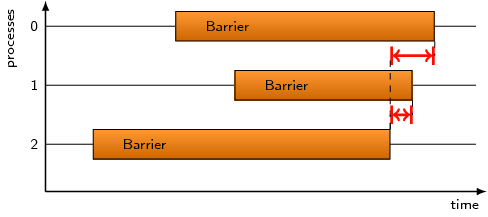
This pattern refers to the time spent in MPI barriers after the first
process has left the operation.
Unit:
Seconds
Diagnosis:
Generally all processes can be expected to leave MPI barriers
simultaneously, and any significant barrier completion time may
indicate an inefficient MPI implementation or interference from other
processes running on the same compute resources.
This pattern refers to the total time spent in MPI point-to-point
communication calls. Note that this is only the respective times for
the sending and receiving calls, and not message transmission
time.
Unit:
Seconds
Diagnosis:
Investigate whether communication time is commensurate with the number
of Communications and Bytes Transferred. Consider replacing blocking
communication with non-blocking communication that can potentially be
overlapped with computation, or using persistent communication to
amortize message setup costs for common transfers. Also consider the
mapping of processes onto compute resources, especially if there are
notable differences in communication time for particular processes,
which might indicate longer/slower transmission routes or network
congestion.
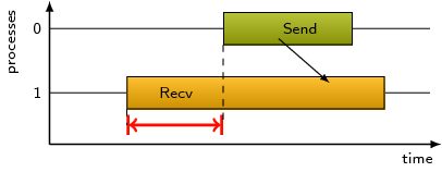
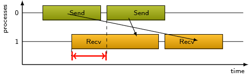
Refers to the time lost waiting caused by a blocking receive operation
(e.g., MPI_Recv or MPI_Wait) that is posted earlier
than the corresponding send operation.
If the receiving process is waiting for multiple messages to arrive
(e.g., in an call to MPI_Waitall), the maximum waiting time is
accounted, i.e., the waiting time due to the latest sender.
Unit:
Seconds
Diagnosis:
Try to replace MPI_Recv with a non-blocking receive MPI_Irecv
that can be posted earlier, proceed concurrently with computation, and
complete with a wait operation after the message is expected to have been sent.
Try to post sends earlier, such that they are available when receivers
need them. Note that outstanding messages (i.e., sent before the
receiver is ready) will occupy internal message buffers, and that large
numbers of posted receive buffers will also introduce message management overhead,
therefore moderation is advisable.
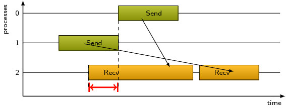
A Late Sender situation may be the result of messages that are received
in the wrong order. If a process expects messages from one or more
processes in a certain order, although these processes are sending them
in a different order, the receiver may need to wait for a message if it
tries to receive a message early that has been sent late.
This pattern comes in two variants:
The messages involved were sent from the same source location
The messages involved were sent from different source locations
See the description of the corresponding specializations for more details.
This specialization of the Late Sender, Wrong Order pattern refers
to wrong order situations due to messages received from the same source
location.
Unit:
Seconds
Diagnosis:
Swap the order of receiving to match the order messages are sent, or
swap the order of sending to match the order they are expected to be
received. Consider using the wildcard MPI_ANY_TAG to receive
(and process) messages in the order they arrive from the source.
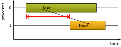
A send operation may be blocked until the corresponding receive
operation is called, and this pattern refers to the time spent waiting
as a result of this situation.
Note that this pattern does currently not apply to nonblocking sends
waiting in the corresponding completion call, e.g., MPI_Wait.
Unit:
Seconds
Diagnosis:
Check the proportion of Point-to-point Send Communications that are Late Receiver Instances (Communications).
The MPI implementation may be working in synchronous mode by default,
such that explicit use of asynchronous nonblocking sends can be tried.
If the size of the message to be sent exceeds the available MPI
internal buffer space then the operation will be blocked until the data
can be transferred to the receiver: some MPI implementations allow
larger internal buffers or different thresholds to be specified. Also
consider the mapping of processes onto compute resources, especially if
there are notable differences in communication time for particular
processes, which might indicate longer/slower transmission routes or
network congestion.
This pattern refers to the total time spent in MPI collective
communication calls.
Unit:
Seconds
Diagnosis:
As the number of participating MPI processes
increase (i.e., ranks in MPI_COMM_WORLD or a subcommunicator),
time in collective communication can be expected to increase
correspondingly. Part of the increase will be due to additional data
transmission requirements, which are generally similar for all
participants. A significant part is typically time some (often many)
processes are blocked waiting for the last of the required participants
to reach the collective operation. This may be indicated by significant
variation in collective communication time across processes, but is
most conclusively quantified from the child metrics determinable via
automatic trace pattern analysis.
Since basic transmission cost per byte for collectives can be relatively high,
combining several collective operations of the same type each with small amounts of data
(e.g., a single value per rank) into fewer operations with larger payloads
using either a vector/array of values or aggregate datatype may be beneficial.
(Overdoing this and aggregating very large message payloads is counter-productive
due to explicit and implicit memory requirements, and MPI protocol switches
for messages larger than an eager transmission threshold.)
MPI implementations generally provide optimized collective communication operations,
however, in rare cases, it may be appropriate to replace a collective
communication operation provided by the MPI implementation with a
customized implementation of your own using point-to-point operations.
For example, certain MPI implementations of MPI_Scan include
unnecessary synchronization of all participating processes, or
asynchronous variants of collective operations may be preferable to
fully synchronous ones where they permit overlapping of computation.
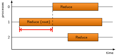
Collective communication operations that send data from all processes
to one destination process (i.e., n-to-1) may suffer from waiting times
if the destination process enters the operation earlier than its
sending counterparts, that is, before any data could have been sent.
The pattern refers to the time lost as a result of this situation. It
applies to the MPI calls MPI_Reduce, MPI_Gather and
MPI_Gatherv.
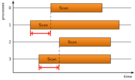
MPI_Scan or MPI_Exscan operations may suffer from
waiting times if the process with rank n enters the operation
earlier than its sending counterparts (i.e., ranks 0..n-1). The
pattern refers to the time lost as a result of this situation.
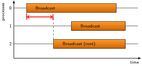
Collective communication operations that send data from one source
process to all processes (i.e., 1-to-n) may suffer from waiting times
if destination processes enter the operation earlier than the source
process, that is, before any data could have been sent. The pattern
refers to the time lost as a result of this situation. It applies to
the MPI calls MPI_Bcast, MPI_Scatter and
MPI_Scatterv.
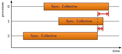
Collective communication operations that send data from all processes
to all processes (i.e., n-to-n) exhibit an inherent synchronization
among all participants, that is, no process can finish the operation
until the last process has started it. This pattern covers the time
spent in n-to-n operations until all processes have reached it. It
applies to the MPI calls MPI_Reduce_scatter,
MPI_Reduce_scatter_block, MPI_Allgather,
MPI_Allgatherv, MPI_Allreduce and MPI_Alltoall.
Note that the time reported by this pattern is not necessarily
completely waiting time since some processes could – at least
theoretically – already communicate with each other while others
have not yet entered the operation.
This pattern refers to the time spent in MPI n-to-n collectives after
the first process has left the operation.
Note that the time reported by this pattern is not necessarily
completely waiting time since some processes could – at least
theoretically – still communicate with each other while others
have already finished communicating and exited the operation.
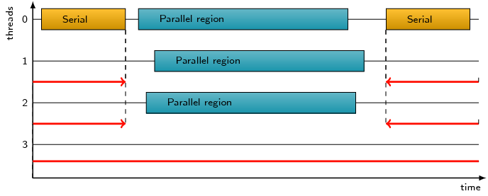
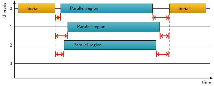
Idle time on CPUs that may be reserved for teams of threads when the
process is executing sequentially before and after OpenMP parallel
regions, or with less than the full team within OpenMP parallel
regions.
Unit:
Seconds
Diagnosis:
On shared compute resources, unused threads may simply sleep and allow
the resources to be used by other applications, however, on dedicated
compute resources (or where unused threads busy-wait and thereby occupy
the resources) their idle time is charged to the application.
According to Amdahl's Law, the fraction of inherently serial execution
time limits the effectiveness of employing additional threads to reduce
the execution time of parallel regions. Where the Idle Threads Time is
significant, total Time (and wall-clock execution time) may be
reduced by effective parallelization of sections of code which execute
serially. Alternatively, the proportion of wasted Idle Threads Time
will be reduced by running with fewer threads, albeit resulting in a
longer wall-clock execution time but more effective usage of the
allocated compute resources.
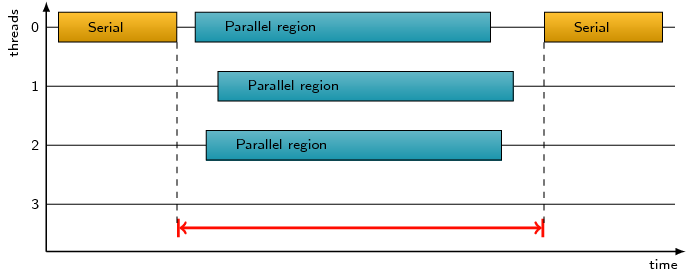
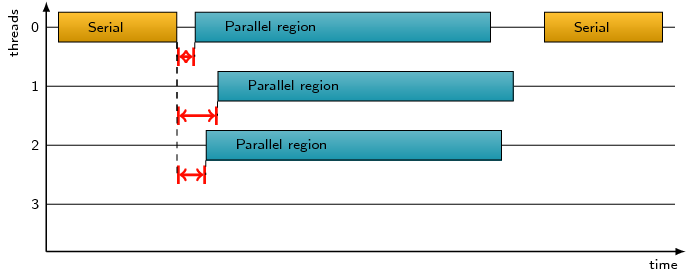
Idle time on CPUs that may be reserved for threads within OpenMP
parallel regions where not all of the thread team participates.
Unit:
Seconds
Diagnosis:
Code sections marked as OpenMP parallel regions which are executed
serially (i.e., only by the master thread) or by less than the full
team of threads, can result in allocated but unused compute resources
being wasted. Typically this arises from insufficient work being
available within the marked parallel region to productively employ all
threads. This may be because the loop contains too few iterations or
the OpenMP runtime has determined that additional threads would not be
productive. Alternatively, the OpenMP omp_set_num_threads API
or num_threads or if clauses may have been explicitly
specified, e.g., to reduce parallel execution overheads such as
OpenMP Management Time or OpenMP Synchronization Time. If the proportion of
OpenMP Limited parallelism Time is significant, it may be more
efficient to run with fewer threads for that problem size.
Time spent managing teams of threads, creating and initializing them
when forking a new parallel region and clearing up afterwards when
joining.
Unit:
Seconds
Diagnosis:
Management overhead for an OpenMP parallel region depends on the number
of threads to be employed and the number of variables to be initialized
and saved for each thread, each time the parallel region is executed.
Typically a pool of threads is used by the OpenMP runtime system to
avoid forking and joining threads in each parallel region, however,
threads from the pool still need to be added to the team and assigned
tasks to perform according to the specified schedule. When the overhead
is a significant proportion of the time for executing the parallel
region, it is worth investigating whether several parallel regions can
be combined to amortize thread management overheads. Alternatively, it
may be appropriate to reduce the number of threads either for the
entire execution or only for this parallel region (e.g., via
num_threads or if clauses).
Time spent in OpenMP synchronization, whether barriers or mutual exclusion
via ordered sequentialization, critical sections, atomics or lock API calls.
Time spent in implicit (compiler-generated)
or explicit (user-specified) OpenMP barrier synchronization. Note that
during measurement implicit barriers are treated similar to explicit
ones. The instrumentation procedure replaces an implicit barrier with an
explicit barrier enclosed by the parallel construct. This is done by
adding a nowait clause and a barrier directive as the last statement of
the parallel construct. In cases where the implicit barrier cannot be
removed (i.e., parallel region), the explicit barrier is executed in
front of the implicit barrier, which will then be negligible because the
team will already be synchronized when reaching it. The synthetic
explicit barrier appears as a special implicit barrier construct.
Time spent in explicit (i.e., user-specified) OpenMP barrier
synchronization, both waiting for other threads Wait at Explicit OpenMP Barrier Time
and inherent barrier processing overhead.
Unit:
Seconds
Diagnosis:
Locate the most costly barrier synchronizations and determine whether
they are necessary to ensure correctness or could be safely removed
(based on algorithm analysis). Consider replacing an explicit barrier
with a potentially more efficient construct, such as a critical section
or atomic, or use explicit locks. Examine the time that each thread
spends waiting at each explicit barrier, and try to re-distribute
preceding work to improve load balance.
Time spent in explicit (i.e., user-specified) OpenMP barrier
synchronization waiting for the last thread.
Unit:
Seconds
Diagnosis:
A large amount of waiting time at barriers can be an indication of load
imbalance. Examine the waiting times for each thread and try to
distribute the preceding computation from threads with the shortest
waiting times to those with the longest waiting times.
Time spent in implicit (i.e., compiler-generated) OpenMP barrier
synchronization, both waiting for other threads Wait at Implicit OpenMP Barrier Time
and inherent barrier processing overhead.
Unit:
Seconds
Diagnosis:
Examine the time that each thread spends waiting at each implicit
barrier, and if there is a significant imbalance then investigate
whether a schedule clause is appropriate. Note that
dynamic and guided schedules may require more
OpenMP Management Time than static schedules. Consider whether
it is possible to employ the nowait clause to reduce the
number of implicit barrier synchronizations.
Time spent in implicit (i.e., compiler-generated) OpenMP barrier
synchronization.
Unit:
Seconds
Diagnosis:
A large amount of waiting time at barriers can be an indication of load
imbalance. Examine the waiting times for each thread and try to
distribute the preceding computation from threads with the shortest
waiting times to those with the longest waiting times.
Time spent waiting to enter OpenMP critical sections and in atomics,
where mutual exclusion restricts access to a single thread at a time.
Unit:
Seconds
Diagnosis:
Locate the most costly critical sections and atomics and determine
whether they are necessary to ensure correctness or could be safely
removed (based on algorithm analysis).
Time spent in OpenMP API calls dealing with locks.
Unit:
Seconds
Diagnosis:
Locate the most costly usage of locks and determine whether they are
necessary to ensure correctness or could be safely removed (based on
algorithm analysis). Consider re-writing the algorithm to use lock-free
data structures.
Time spent waiting to enter OpenMP ordered regions due to enforced
sequentialization of loop iteration execution order in the region.
Unit:
Seconds
Diagnosis:
Locate the most costly ordered regions and determine
whether they are necessary to ensure correctness or could be safely
removed (based on algorithm analysis).
This metric provides the total number of MPI synchronization operations
that were executed. This not only includes barrier calls, but also
communication operations which transfer no data (i.e., zero-sized
messages are considered to be used for coordination synchronization).
The total number of MPI point-to-point synchronization
operations, i.e., point-to-point transfers of zero-sized messages used
for coordination.
Unit:
Counts
Diagnosis:
Locate the most costly synchronizations and determine whether they are
necessary to ensure correctness or could be safely removed (based on
algorithm analysis).
The number of MPI collective synchronization operations. This
does not only include barrier calls, but also calls to collective
communication operations that are neither sending nor receiving any
data. Each process participating in the operation is counted, as
defined by the associated MPI communicator.
Unit:
Counts
Diagnosis:
Locate synchronizations with the largest MPI Collective Synchronization Time and
determine whether they are necessary to ensure correctness or could be
safely removed (based on algorithm analysis). Collective communication
operations that neither send nor receive data, yet are required for
synchronization, can be replaced with the more efficient
MPI_Barrier.
The number of MPI collective communication operations, excluding
calls neither sending nor receiving any data. Each process participating
in the operation is counted, as defined by the associated MPI communicator.
Unit:
Counts
Diagnosis:
Locate operations with the largest MPI Collective Communication Time and compare Collective Bytes Transferred.
Where multiple collective operations of the same type are used in series with single
values or small payloads, aggregation may be beneficial in amortizing transfer overhead.
The number of MPI collective communication operations which are
both sending and receiving data. In addition to all-to-all and scan operations,
root processes of certain collectives transfer data from their source to
destination buffer.
The number of MPI collective communication operations that are
only sending but not receiving data. Examples are the non-root
processes in gather and reduction operations.
The number of MPI collective communication operations that are
only receiving but not sending data. Examples are broadcasts
and scatters (for ranks other than the root).
The total number of bytes that were notionally processed in
MPI communication operations (i.e., the sum of the bytes that were sent
and received). Note that the actual number of bytes transferred is
typically not determinable, as this is dependant on the MPI internal
implementation, including message transfer and failed delivery recovery
protocols.
Unit:
Bytes
Diagnosis:
Expand the metric tree to break down the bytes transferred into
constituent classes. Expand the call tree to identify where most data
is transferred and examine the distribution of data transferred by each
process.
The total number of bytes that were notionally processed by
MPI point-to-point communication operations.
Unit:
Bytes
Diagnosis:
Expand the calltree to identify where the most data is transferred
using point-to-point communication and examine the distribution of data
transferred by each process. Compare with the number of Point-to-point Communications
and resulting MPI Point-to-point Communication Time.
Average message size can be determined by dividing by the number of MPI
Point-to-point Communications (for all call paths or for particular call paths or
communication operations). Instead of large numbers of small
communications streamed to the same destination, it may be more
efficient to pack data into fewer larger messages (e.g., using MPI
datatypes). Very large messages may require a rendez-vous between
sender and receiver to ensure sufficient transmission and receipt
capacity before sending commences: try splitting large messages into
smaller ones that can be transferred asynchronously and overlapped with
computation. (Some MPI implementations allow tuning of the rendez-vous
threshold and/or transmission capacity, e.g., via environment
variables.)
If the aggregatePoint-to-point Bytes Received is less than the amount
sent, some messages were cancelled, received into buffers which were
too small, or simply not received at all. (Generally only aggregate
values can be compared, since sends and receives take place on
different callpaths and on different processes.) Sending more data than
is received wastes network bandwidth. Applications do not conform to
the MPI standard when they do not receive all messages that are sent,
and the unreceived messages degrade performance by consuming network
bandwidth and/or occupying message buffers. Cancelling send operations
is typically expensive, since it usually generates one or more internal
messages.
If the aggregatePoint-to-point Bytes Sent is greater than the amount
received, some messages were cancelled, received into buffers which
were too small, or simply not received at all. (Generally only
aggregate values can be compared, since sends and receives take place
on different callpaths and on different processes.) Applications do
not conform to the MPI standard when they do not receive all messages
that are sent, and the unreceived messages degrade performance by
consuming network bandwidth and/or occupying message buffers.
Cancelling receive operations may be necessary where speculative
asynchronous receives are employed, however, managing the associated
requests also involves some overhead.
The total number of bytes that were notionally processed in
MPI collective communication operations. This assumes that collective
communications are implemented naively using point-to-point
communications, e.g., a broadcast being implemented as sends to each
member of the communicator (including the root itself). Note that
effective MPI implementations use optimized algorithms and/or special
hardware, such that the actual number of bytes transferred may be very
different.
Unit:
Bytes
Diagnosis:
Expand the calltree to see where the most data is transferred using
collective communication and examine the distribution of data
transferred by each process. Compare with the number of
Collective Communications and resulting MPI Collective Communication Time.
The number of bytes that were notionally sent by MPI
collective communication operations.
Unit:
Bytes
Diagnosis:
Expand the calltree to see where the most data is transferred using
collective communication and examine the distribution of data outgoing
from each process.
The number of bytes that were notionally received by MPI
collective communication operations.
Unit:
Bytes
Diagnosis:
Expand the calltree to see where the most data is transferred using
collective communication and examine the distribution of data incoming
to each process.
Provides the total number of Late Sender instances found in
point-to-point communication operations were messages where sent in
wrong order (see also Late Sender, Wrong Order Time).
Provides the total number of Late Sender instances (see
Late Sender Time for details) found in point-to-point
synchronization operations (i.e., zero-sized message transfers).
Provides the total number of Late Sender instances found in
point-to-point synchronization operations (i.e., zero-sized message
transfers) where messages are received in wrong order (see also
Late Sender, Wrong Order Time).
Provides the total number of Late Receiver instances (see
Late Receiver Time for details) found in point-to-point
synchronization operations (i.e., zero-sized message transfers).
Expand the metric tree to see the breakdown of different classes of MPI
file operation, expand the calltree to see where they occur, and look
at the distribution of operations done by each process.
Compare with the corresponding number of MPI File Bytes Transferred.
Examine the callpaths where individual MPI file reads occur and the
distribution of operations done by each process in them, and compare with
the corresponding number of MPI File Individual Bytes Read.
Examine the callpaths where individual MPI file writes occur and the
distribution of operations done by each process in them, and compare with
the corresponding number of MPI File Individual Bytes Written.
Examine the callpaths where collective MPI file reads occur and the
distribution of operations done by each process in them, and compare with
the corresponding number of MPI File Collective Bytes Read.
Examine the callpaths where collective MPI file writes occur and the
distribution of operations done by each process in them, and compare with
the corresponding number of MPI File Collective Bytes Written.
Number of bytes read or written in MPI file operations of any type.
Unit:
Bytes
Diagnosis:
Expand the metric tree to see the breakdown of different classes of MPI
file operation, expand the calltree to see where they occur, and look
at the distribution of bytes transferred by each process.
Compare with the corresponding number of MPI File Operations.
Number of bytes read or written in individual MPI file operations.
Unit:
Bytes
Diagnosis:
Examine the distribution of bytes transferred in individual MPI file operations done by each
process and compare with the corresponding number of MPI File Individual Operations
and resulting exclusiveMPI File I/O Time.
Number of bytes read in individual MPI file operations.
Unit:
Bytes
Diagnosis:
Examine the callpaths where individual MPI file reads occur and the
distribution of bytes read by each process in them, and compare with
the corresponding number of MPI File Individual Read Operations.
Number of bytes written in individual MPI file operations.
Unit:
Bytes
Diagnosis:
Examine the callpaths where individual MPI file writes occur and the
distribution of bytes written by each process in them, and compare with
the corresponding number of MPI File Individual Write Operations.
Number of bytes read in collective MPI file operations.
Unit:
Bytes
Diagnosis:
Examine the callpaths where collective MPI file reads occur and the
distribution of bytes read by each process in them, and compare with
the corresponding number of MPI File Collective Read Operations.
Number of bytes written in collective MPI file operations.
Unit:
Bytes
Diagnosis:
Examine the callpaths where collective MPI file writes occur and the
distribution of bytes written by each process in them, and compare with
the corresponding number of MPI File Collective Write Operations.
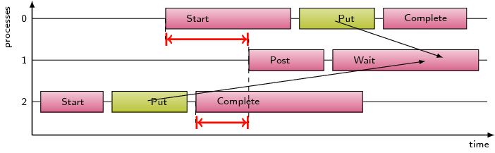
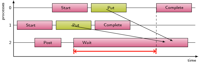
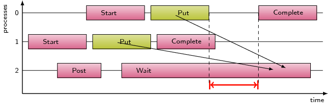
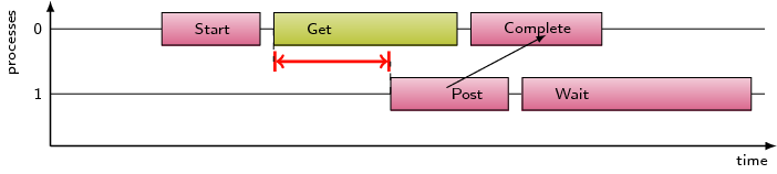
This pattern refers to the time spent waiting in MPI remote memory access
communication routines, i.e. MPI_Accumulate, MPI_Put, and MPI_Get, due to
an access before the exposure epoch is opened at the target.
This pattern refers to the number of pairwise synchronizations done
with MPI RMA active target synchronization mechanisms that do not
complete rma operations.
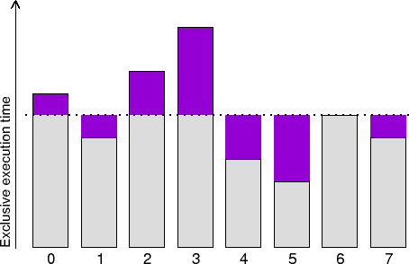
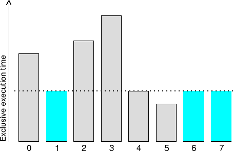
This simple heuristic allows to identify computational load imbalances and
is calculated for each (call-path, process/thread) pair. Its value
represents the absolute difference to the average exclusive execution
time. This average value is the aggregated exclusive time spent by all
processes/threads in this call-path, divided by the number of
processes/threads visiting it.
Note:
A high value for a collapsed call tree node does not necessarily mean that
there is a load imbalance in this particular node, but the imbalance can
also be somewhere in the subtree underneath. Unused threads outside
of OpenMP parallel regions are considered to constitute OpenMP Idle threads Time
and expressly excluded from the computational load imbalance heuristic.
Unit:
Seconds
Diagnosis:
Total load imbalance comprises both above average computation time
and below average computation time, therefore at most half of it could
potentially be recovered with perfect (zero-overhead) load balance
that distributed the excess from overloaded to unloaded
processes/threads, such that all took exactly the same time.
Computation imbalance is often the origin of communication and
synchronization inefficiencies, where processes/threads block and
must wait idle for partners, however, work partitioning and
parallelization overheads may be prohibitive for complex computations
or unproductive for short computations. Replicating computation on
all processes/threads will eliminate imbalance, but would typically
not result in recover of this imbalance time (though it may reduce
associated communication and synchronization requirements).
Call-paths with significant amounts of computational imbalance should
be examined, along with processes/threads with above/below-average
computation time, to identify parallelization inefficiencies. Call-paths
executed by a subset of processes/threads may relate to parallelization
that hasn't been fully realized (Computational load imbalance heuristic (non-participation)), whereas
call-paths executed only by a single process/thread
(Computational load imbalance heuristic (single participant)) often represent unparallelized serial code,
which will be scalability impediments as the number of processes/threads
increase.
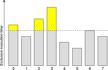
This metric identifies processes/threads where the exclusive execution
time spent for a particular call-path was above the average value.
It is a complement to Computational load imbalance heuristic (underload).
The CPU time which is above the average time for computation is the
maximum that could potentially be recovered with perfect (zero-overhead)
load balance that distributed the excess from overloaded to underloaded
processes/threads.
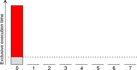
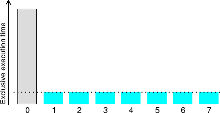
This heuristic distinguishes the execution time for call-paths executed
by single processes/threads that potentially could be recovered with
perfect parallelization using all available processes/threads.
This time is often associated with activities done exclusively by a
"Master" process/thread (often rank 0) such as initialization,
finalization or I/O, but can apply to any process/thread that
performs computation that none of its peers do (or that does its
computation on a call-path that differs from the others).
The CPU time for singular execution of the particular call-path
typically presents a serial bottleneck impeding scalability as none of
the other available processes/threads are being used, and
they may well wait idling until the result of this computation becomes
available. (Check the MPI communication and synchronization times,
particularly waiting times, for proximate call-paths.)
In such cases, even small amounts of singular execution can
have substantial impact on overall performance and parallel efficiency.
With perfect partitioning and (zero-overhead) parallel
execution of the computation, it would be possible to recover this time.
When the amount of time is small compared to the total execution time,
or when the cost of parallelization is prohibitive, it may not be
worth trying to eliminate this inefficiency. As the number of
processes/threads are increased and/or total execution time decreases,
however, the relative impact of this inefficiency can be expected to grow.
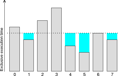
This metric identifies processes/threads where the exclusive execution
time spent for a particular call-path was below the average value.
It is a complement to Computational load imbalance heuristic (overload).
The CPU time which is below the average time for computation could
potentially be used to reduce the excess from overloaded processes/threads
with perfect (zero-overhead) load balancing.
This heuristic distinguishes the execution time for call-paths not executed
by a subset of processes/threads that potentially could be used with
perfect parallelization using all available processes/threads.
The CPU time used for call-paths where not all processes or threads
are exploited typically presents an ineffective parallelization that
limits scalability, if the unused processes/threads wait idling for
the result of this computation to become available. With perfect
partitioning and (zero-overhead) parallel execution of the computation,
it would be possible to recover this time.
This heuristic distinguishes the execution time for call-paths not executed
by all but a single process/thread that potentially could be recovered with
perfect parallelization using all available processes/threads.
The CPU time for singular execution of the particular call-path
typically presents a serial bottleneck impeding scalability as none of
the other processes/threads that are available are being used, and
they may well wait idling until the result of this computation becomes
available. With perfect partitioning and (zero-overhead) parallel
execution of the computation, it would be possible to recover this time.